
A preliminary HelioLinC based pipeline for CSS data
UPDATE: When I initially published this study I mistakenly used CSS .dets files as the source for their candidate links. I later learned that the .dets file shows only a subset of CSS' candidate links and that the full set of CSS candidate links is produced in the .mtds file. I've updated the study and all of the results below using the .mtds comparison.
In this study I use real observational data from Catalina Sky Survey's 1.5m telescope on Mountain Lemmon (G96) and process it with a preliminary version of a HelioLinC based pipeline I'm developing to find solar system objects in their data. To my surprise, I was able to link 7 additional known objects beyond what CSS linked. Below I'll review the 3 main parts of this new pipeline and detail the results it generates for G96 field N18061 observations on 2/1/2022.
Part 1: Data reduction
CSS has an interesting and unique (as far as I know) method for generating source detections from observations. Like a lot of other surveys, CSS creates difference images that highlight what's changed between repeat observations of the same field. But CSS also extracts all sources from each individual observation. This data necessarily includes many stellar sources but doesn't require a high quality template image like difference imaging does to produce — you simply note the location and brightness of all points of light that register on the CCD for each observation all the way down to the limiting magnitude of the hardware. CSS then combines both of these sets of data and can link more objects as a result than with either technique alone.
For this study I consider only the sources from the non-difference imaging data. Difference imaging data is definitely worth using, I just haven't implemented a method to process it yet. I'll refer to this non-difference image data as sext sources as it's data from the Source Extractor software that CSS uses. While I won't be using them, I refer to the difference image sources as iext sources because that's what CSS calls them (I think).
Catalina takes four pictures of the same region sky separated by 7-8 minutes over approximately 30 minutes. From these four images Source Extractor produces 258,553 sources for field N18061 on the night of 2/1/2022. These sources include all things from stars and asteroids to bad pixels, planes and satellites passing through the field. The first job for the pipeline is to reduce this number of raw detections by removing sources that are not associated with moving objects in the solar system. In this study I take a very naive but effective (I think) approach to removing the sources we aren't interested in. I simply remove sources that occur more than once in the same location for the four images within a specified location deviation tolerance. This removes sources that repeat in the same spot, mostly stars and bad pixels.
Using a separation tolerance of 0.95" for source de-duping I can reduce the number of sources from 258,553 to 71,993. Why did I choose 0.95" for the de-dupe tolerance? That's the separation one step before I started dropping individual detections of known objects as validated by SBIdent. I simply counted the raw individual sources that match known objects in the unmodified sext data and then began increasing the de-dupe separation tolerance until that count started to decrease. When it did, I backed off one step. The two images below show the results of the de-duping.

Image 1. All 258,553 raw sext sources produced by Catalina Sky Survey for 4 observations of field N18061 on 2/1/2022. Individual sources are plotted with some alpha blending so sources that are plotted on top of one another appear darker.

Image 2. The 71,993 sources that remain after de-duping the raw sext sources in Image 1 within 0.95" of one another. These are the sources that are the input for HelioLinC.
As an aside, there are two ways that I can think of to do this source de-duping. One is to grid the field at some level of resolution, say 1", then remove all sources that occur more than once in each bin. That's what I was doing originally because it's very fast, but there are edge effects with the grid binning methods that allow sources with small separations to end up in separate bins and vice-versa. Thus in the end I implemented a more effective method that tests all sources against all other sources and eliminates any that have a separation less than specified. It's slower, but with a KDTree implementation it's very manageable.
Part 2: Linking with HelioLinC
CSS has developed a robust, fast and effective linking algorithm with a high signal-to-noise ratio. There's really no hope that the naive linker I was using with TESS that tries to discover objects moving at constant-ish on-sky velocities could perform nearly as well as the tools they've built. Their linker is essentially a way more sophisticated version of mine. My HelioLinC implementation, however, is a conceptually different approach to the linking problem and at least offers the hope of getting different results. The HelioLinC NEO study I did with synthetic data also suggests that HelioLinC can find stuff at CSS' cadence, so that's what I've used here.
With HelioLinC there are two categories of parameters to tune for moving object detection: physical parameters and clustering parameters. I won't enumerate all the parameters I chose here, I just want to note some of the 'dials' that I was turning to produce these results.
The primary physical parameters for HelioLinC are the range, range-rate guess you provide. The most obvious thing to do is to provide HelioLinC with range and range-rate guesses that are close to the actual range and range-rates of the objects you're observing (which is not something you know apriori). But as I continually find, non-realistic range and range-rate parameters can often yield more complete results — at least for CSS' cadence. Anyway, for this study I found the best results by using one range and range-rate combination guess: 1.05 AU and 0.02 AU/day respectively.
This is the first study where I felt like I really learned how to tune HelioLinC. By that I mean I was able to adjust the physical and clustering parameters in an intuitive way to increase the number of good linkages I was able to recover and decrease the erroneous ones. The primary dials I was turning for this were clustering parameters: separation tolerance, the maximum tracklets in a cluster and the weighting of the velocity component of the propagated tracklet in the clustering phase space.
With modest tuning, HelioLinC found 2,005 candidate links. Among those 2,005 candidates HelioLinC found were links for 330 out of 330 known objects that were linkable, meaning, there were at least 3 detections of the object in the sext source data within 1" of the known object position at the time of observation as confirmed by SBIdent. So HelioLinC was able to recover 100% of the linkable objects in the sext data. However, 2,005 candidate links is more than I'd like to see. CSS produced only 447 candidate links for the field with sext data (though did not match all 330 possible links). Ideally HelioLinC would discover only 330 links if there were only 330 linkable objects in the observed region of the sky. In the next section I'll explore a way to filter these candidate links further to discard some of the more physically implausible ones.
Part 3: Orbit Determination as a filter
Solar system object detection is a process of finding enough source detections over time to describe a singular object on a well defined orbit. In theory you only need 3 detections at 3 times to fit an orbit to your observations. In practice, however, this is insufficient. Observation error and (in the case of CSS) the short (30 minute) observation time span make any orbit you might fit to your observations unreliable. There are simply too many viable orbits that can fit the small set of observations. However, not finding any orbit that fits your observations is a signal that your candidate link is not physical — it cannot be described by any orbit. Thus I propose using orbit determination as a filter to reject non-physical candidate orbits. We may not have enough data to validate a unique and unvarying orbit, but if we can't find any orbit at all that fits the observations that's useful information too.
For this study I used Find_Orb for orbit determination. I've used OpenOrb previously, but Find_Orb seems to be faster for me and produces more meta data on the orbit solutions it finds. Or maybe I just don't know how to use OpenOrb well enough. Anyway, by sending the 2,005 candidate links that HelioLinC generated to Find_Orb to solve, I was able to reject 1,071 candidate links. I rejected candidate links that couldn't produce an orbit solution with better than 0.5" RMS error. At this RMS rejection threshold no linkages of known objects were rejected, and our candidate links for consideration were reduced by more than half from 2,005 to 934.
With non-physical links filtered, we can consolidate the candidate links that are full subsets of another link. For instance, if there's a link that consists of detections [1,2,3,4] and a link that consists of detections [2,3,4] we can merge the latter into the former since it is a full subset of the longer link. Removing subsets reduces the candidate link count slightly from from 934 to 903.
Results
While I believe there is room to reduce the candidate link set further, for this early work I'll stop here and take 903 as my final set of candidate links. The images below compares my 903 candidate links to the 447 sext-only candidate links that CSS found for the same field on the same night. For an apples-to-apples comparison, I've only shown Catalina candidate links that have 3 or more sext sources. Since I'm not trying to link difference imaging detections yet, I haven't shown CSS' links that require difference image sources to construct.
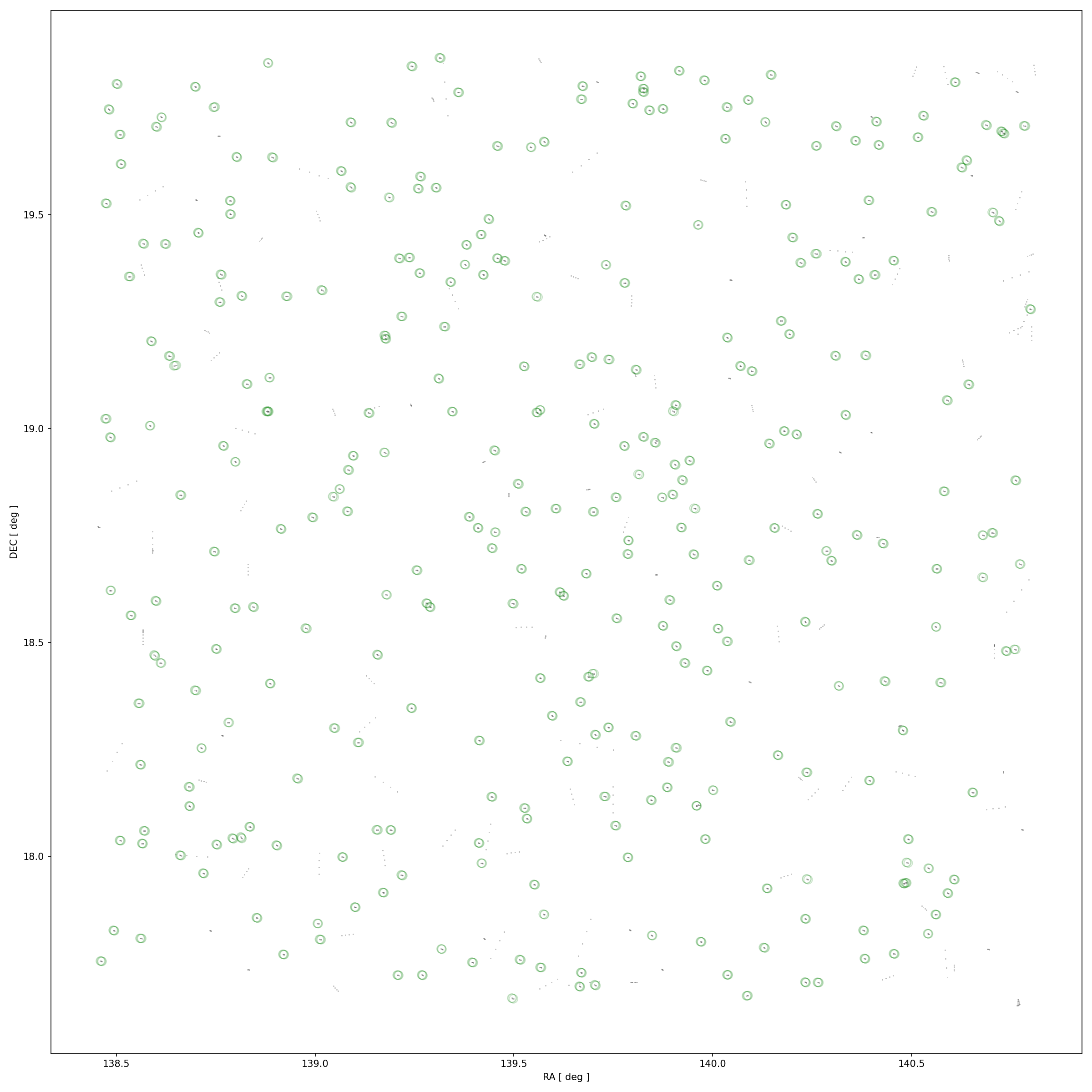
Image 3. Catalina Sky Survey candidate links for field N18061 on 2/1/2022 constructed of 3+ sext sources. Links that match 320 known objects are in green circles.
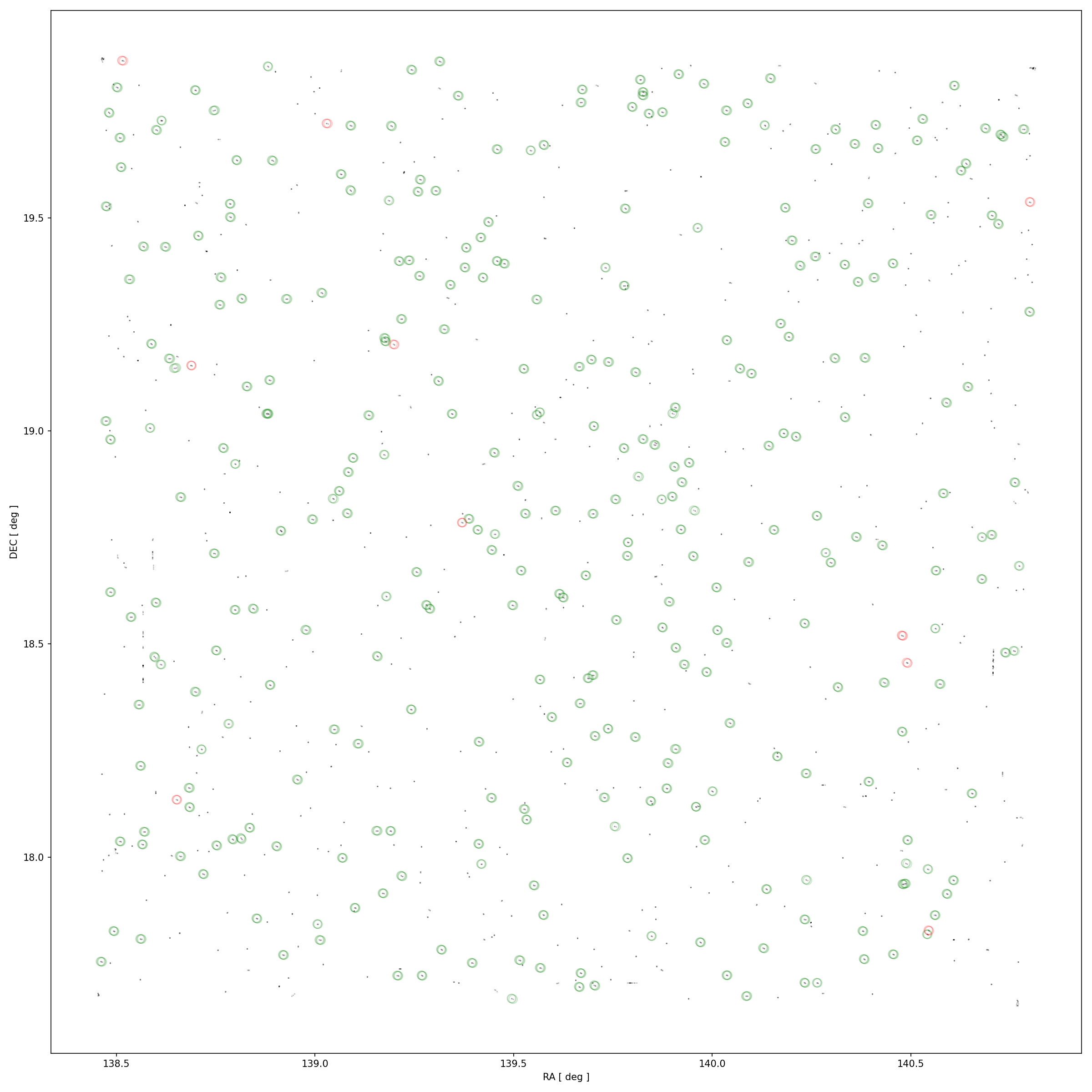
Image 4. HelioLinC generated candidate links for field N18061 on 2/1/2022. Links that match known objects and are also in the set of CSS generated candidate links are in green circles. These are the same 320 links that CSS finds in the sext data. The links in red circles match known objects but are not matched by CSS candidate links in Image 3.
The table below details the 10 linkages of known objects that my HelioLinC pipeline found that did not have a corresponding CSS 3+ sext source based link. These 10 objects are the additional links I matched to known objects in red circles in Image 4 above. Catalina recovered 3 of these 10 objects when difference imaging iext sources were added. However, 7 of these objected were not linked by CSS even when I include their candidate links with iext sources. There were no linkable known objects in the sext-only sources that CSS linked that my pipeline did not link. Also, there were no links that my pipeline could have linked (because there were 3+ sources in the unmodified sext files that matched ephemeris positions) that it did not.
Table 1. Objects linked by the HelioLinC pipeline that weren't linked with CSS sext-only sources
| Linked object |
CSS sext sources in link |
CSS iext sources in link |
HelioLinC sext sources in link |
Object magnitude |
|---|---|---|---|---|
| (2009 UP80) | 2 | 2 | 3 | 20.6 |
| 329550 (2002 TJ342) | 2 | 2 | 3 | 20.7 |
| 431741 (2008 FN123) | 2 | 2 | 4 | 21.3 |
| (2022 BC19) | 0 | 0 | 3 | 21.3 |
| (2008 RU184) | 0 | 0 | 3 | 21.4 |
| (2016 OH10) | 0 | 0 | 3 | 21.6 |
| (2012 UQ2) | 0 | 0 | 3 | 21.7 |
| (2005 QC198) | 0 | 0 | 4 | 21.9 |
| (2019 MW21) | 0 | 0 | 3 | 21.9 |
| (2008 SP18) | 0 | 0 | 3 | 22.2 |
Questions and caveats
I'm still very much getting acquainted with Catalina's data, so while I'm encouraged by these results, I'm aware that I could be making mistakes with my treatment of their observations. Here are a few of the things that stand out to me.
- I've tuned HelioLinC to find as many known objects as it can by mostly using this data. A lot of the potential for a HelioLinC based pipeline depends on whether the tuning parameters I've used remain relatively constant across different fields and nights of observation. Results like this will have to be reproduced many more times before I can get a sense for that.
- HelioLinC tends to work best with observational data of high astrometric accuracy. There might be links that CSS can find that a HelioLinC based linker can't because the source detections are slightly too inaccurate. For instance, CSS might be able to link an object with 2" mean error where HelioLinC may not.
- The (provisional) success of this pipeline may not be due to the linker at all. The data reduction process employed by CSS analagous to 'part 1' of this study is not observable to me. It's possible that the new linkages I'm finding are due to my de-duping strategy rather than anything special that HelioLinC is doing.
- Along those lines, one interesting thing about the results in the table above is that all of my additional linkages are of relatively dim objects. Also, the 3 out of 10 objects that CSS does link require additional iext data and are all on the brighter end of the spectrum. I don't have a good explanation for this. Is CSS explicitly excluding the dimmer sources that constitute these links I'm finding for some reason? The individual sources that make up the links are definitely in the raw sext file and match ephemeris data to less than 1" accuracy.
- Another noteworthy observation from the table of results is that almost all of the additional links I found contain only 3 source detections. I think Catalina sees 3 detection links as valid, but if not then I've not really found as many additional known objects in the data as this study suggests.
Conclusion & next steps
As I said, I'm very encouraged to be linking additional known objects beyond what Catalina is linking. However, I think the biggest flaw in this work is that I'm generating 456 more candidate links than CSS is in order to capture only 7 additional known objects. I have some ideas to reduce that count, but by comparison CSS has developed a linking algorithm with a substantially better signal-to-noise ratio than what my pipeline is producing. They have a human looking at these things every night and a human can only validate so many candidates manually. Therefore, most links have to be real. It's very unlikely that those 456 additional candidates that I'm generating are real linkages, so reducing that number without losing the 7 extra valid links is what I'll be focusing on next. I would also like to develop a set of tools for inspecting the images that CSS captures to visually verify the sources that make up some of these links like Catalina does — at least to verify that the known objects are real detections not fortuitously placed noise or CCD errors.
Published: 6/13/2022; Updated: 6/17/2022