
Detecting Asteroids with TESS - a Preliminary Study
I learned about TESS while attending the LSST Project and Community Workshop in August. Bruno Sanchez, a postdoc at Duke, pointed me towards the Gaia astrometry survey as a potential source of data for this project. It doesn't look like Gaia distributes raw images at this point, but reading about Gaia led to a fortuitous mention of TESS somewhere along the way. TESS is a NASA mission designed to search for exoplanets, but since it observes the same patches of sky over and over again to accomplish this it also works as a source for solar system object detection. And the TESS project distributes calibrated full frame images, so my image processing tools can be applied rather directly to TESS data. TESS can observe approximately 85% of the sky; I think this is going to be a pretty good data source for me.
A few notes regarding presentation below: 1. For each image set I'll have a high level description just below the image and a more detailed technical description for each image set just below the images in the technical details section. 2. Because these images are rather large and the detail small, a desktop or laptop is better than mobile. Make your browser as wide as you can too. 3. I've done some preliminary identification of the objects in these images, but I'm not completely satisfied with my process yet so consider the object identification part very preliminary.
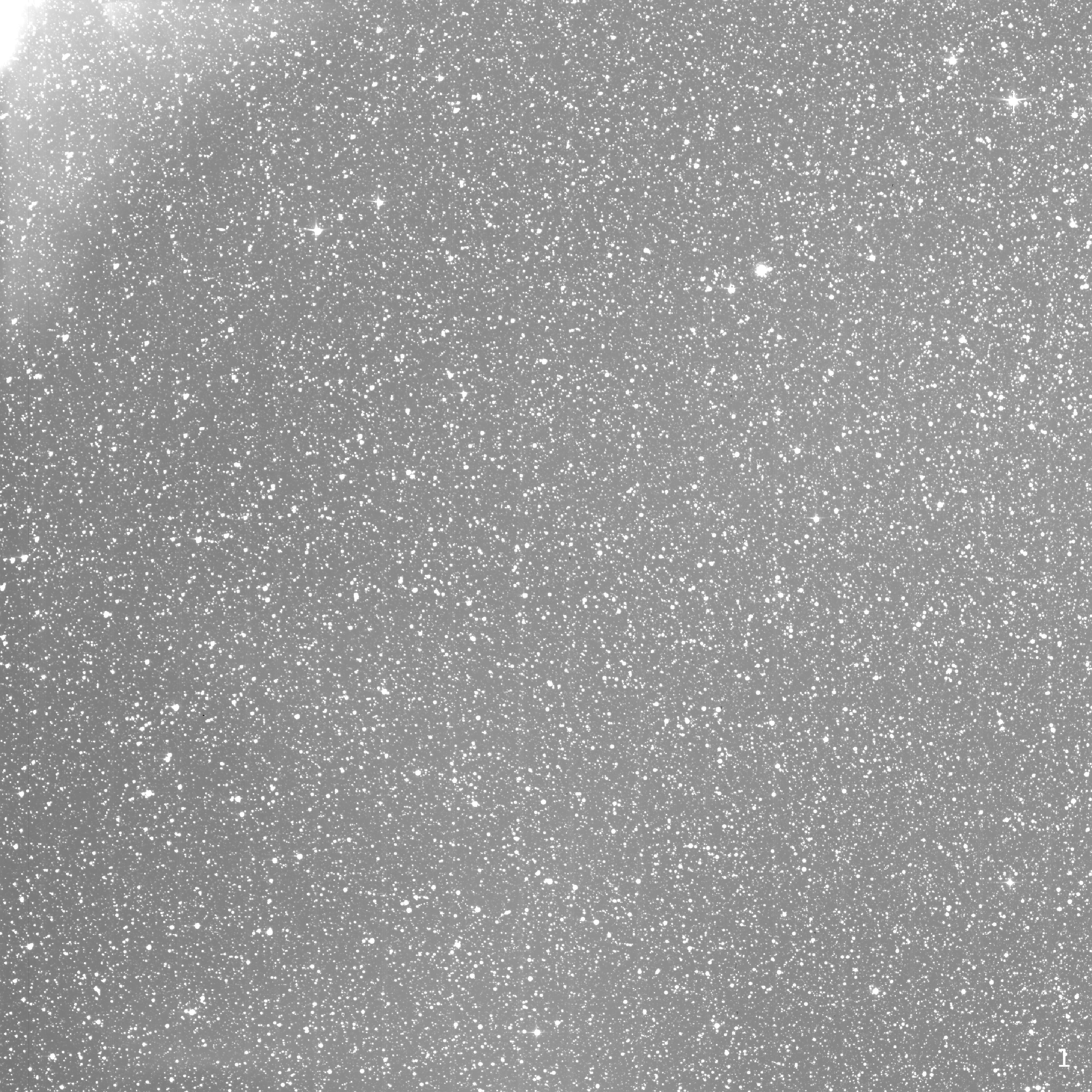
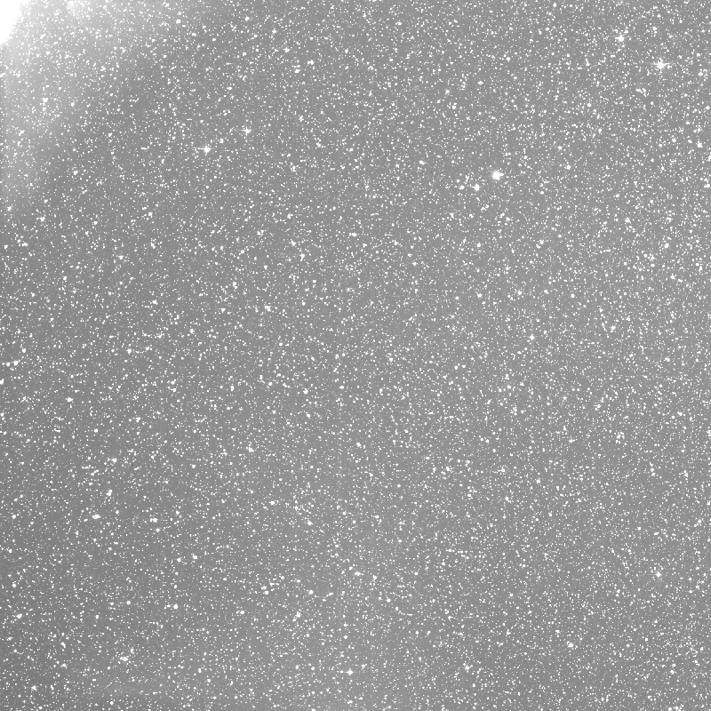
1. This is an animation of 4 TESS frames near the ecliptic between August 16th 2018 and August 20th 2018. These aren't quite original, unmodified TESS images, but they're very close. I've cropped the buffer border pixels with no data and applied brightness matching to the frames. You should be able to make out some movement if you look close enough. I could see 3 or 4 objects which is why I selected this set of observations.
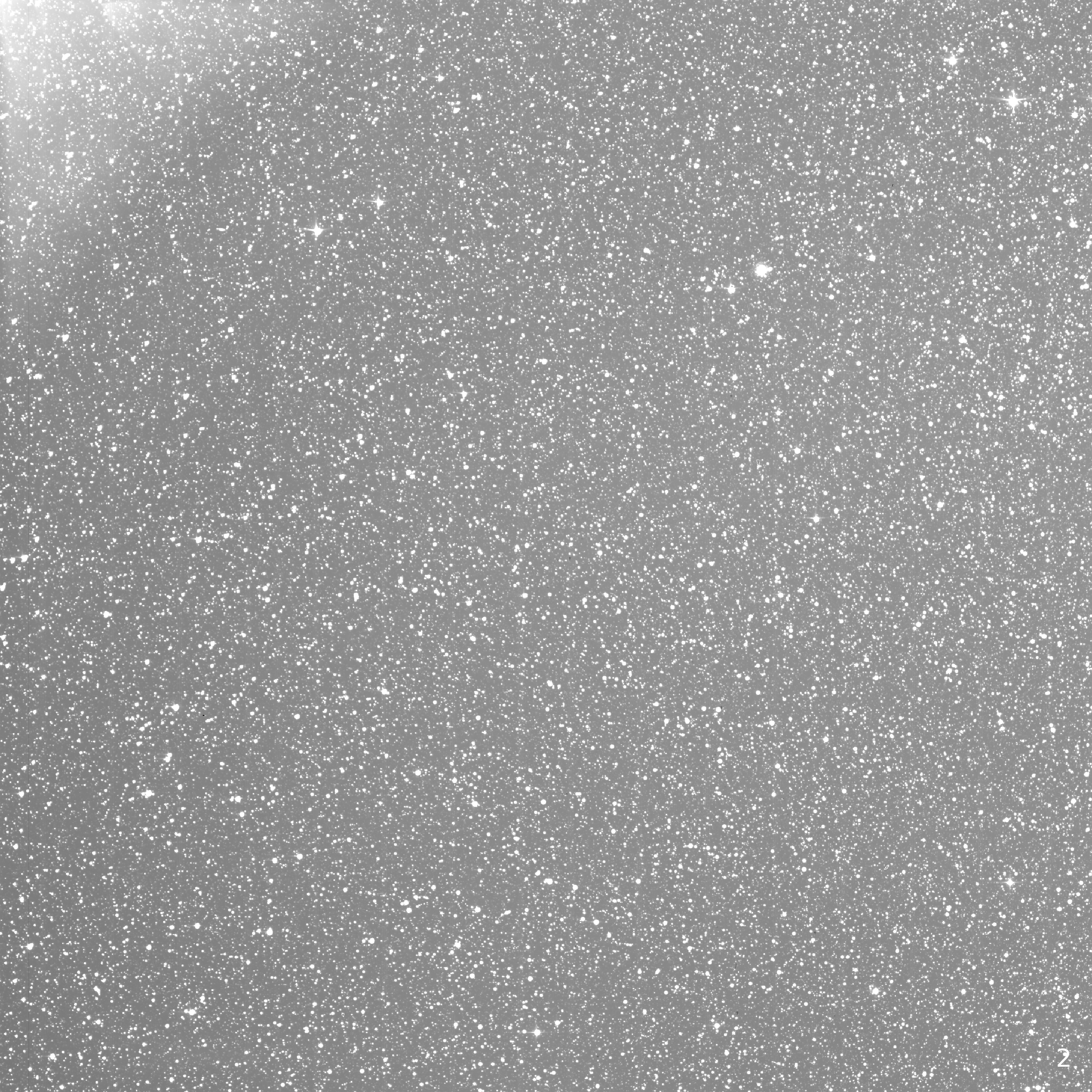
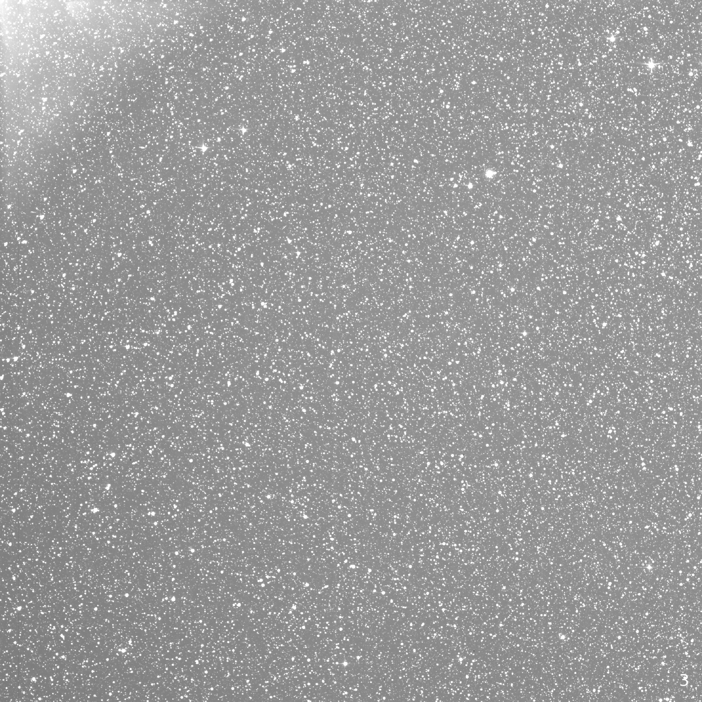
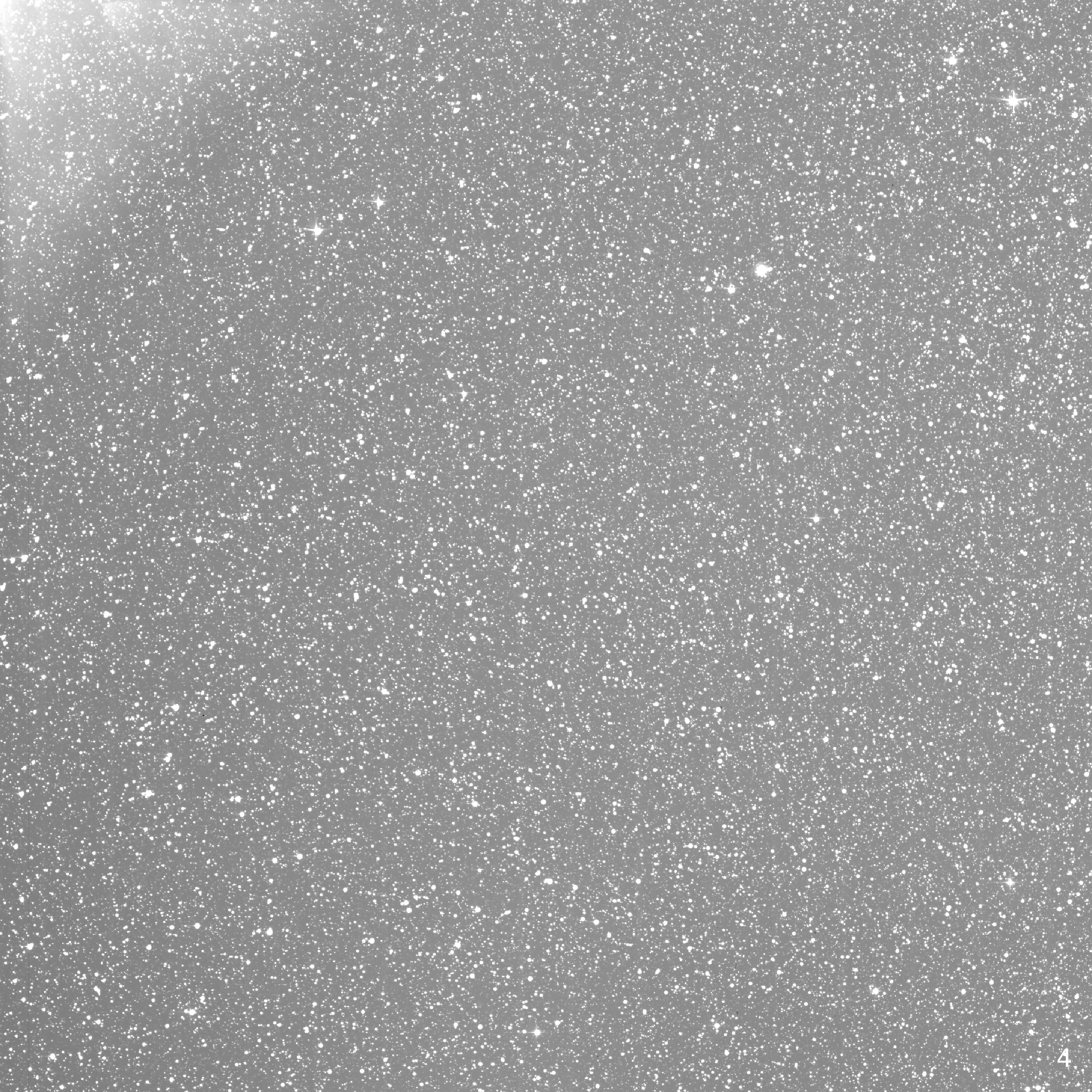
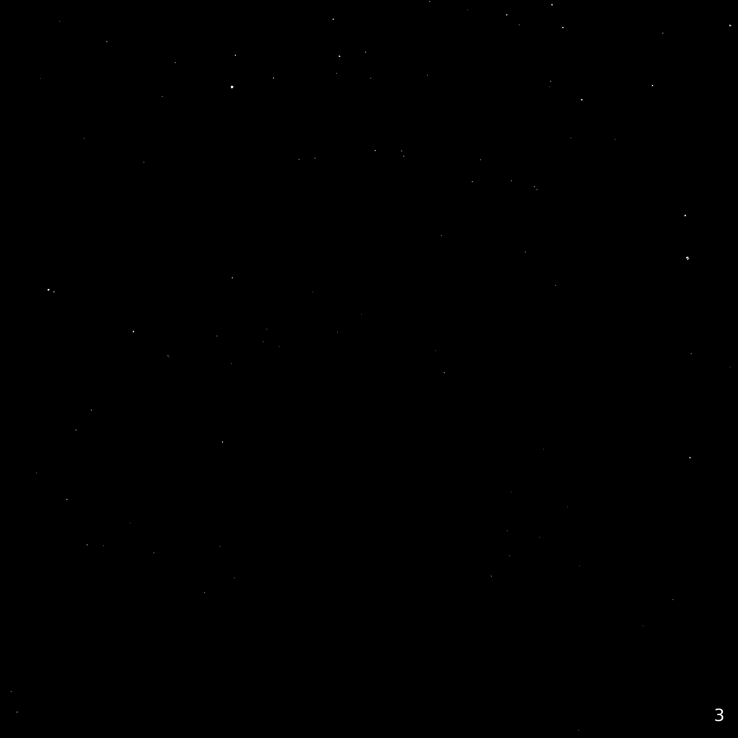
2. This is the static sky template generated (in part) from image set 1. This is a singular image, so don't squint too hard trying to see what's changing.


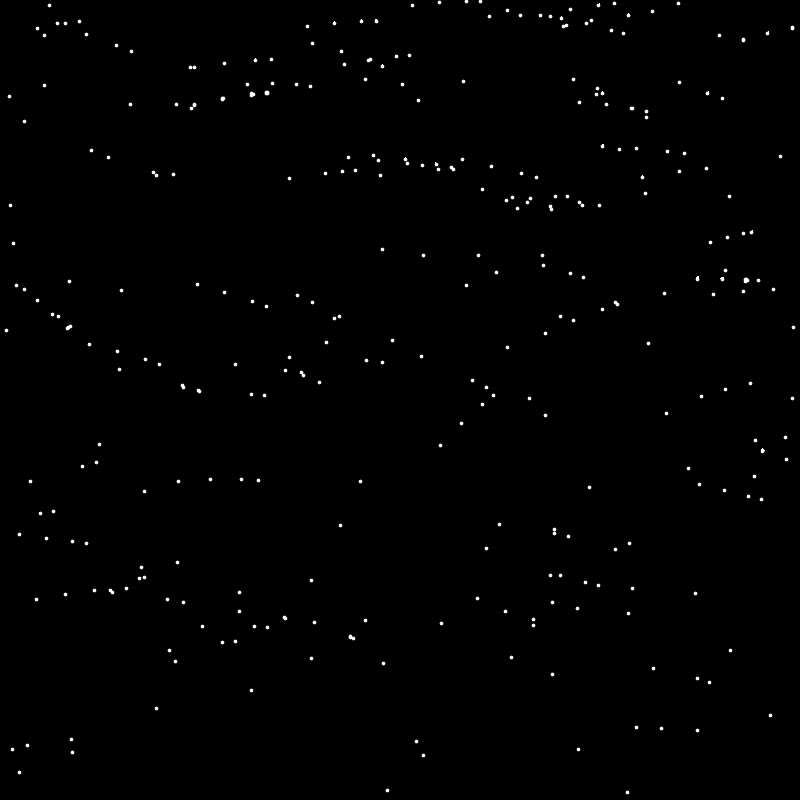
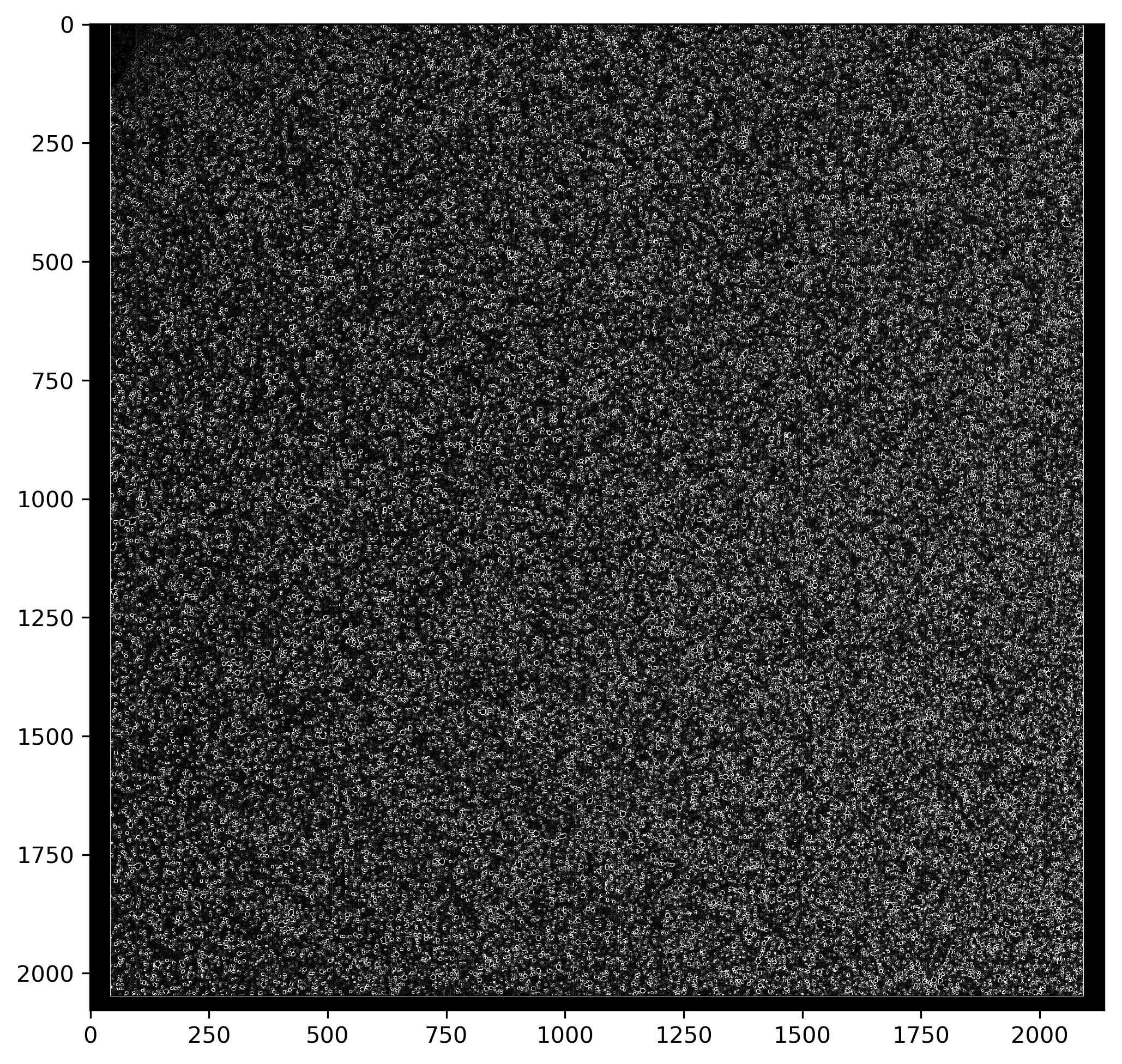
3. These are the difference images generated by subtracting image 2 from each frame of image set 1. Removing the static sky reveals the dynamic sky. The largest objects in these frames correspond to the moving objects I could see in the image set 1 frames, but there are obviously a lot more objects revealed here too.
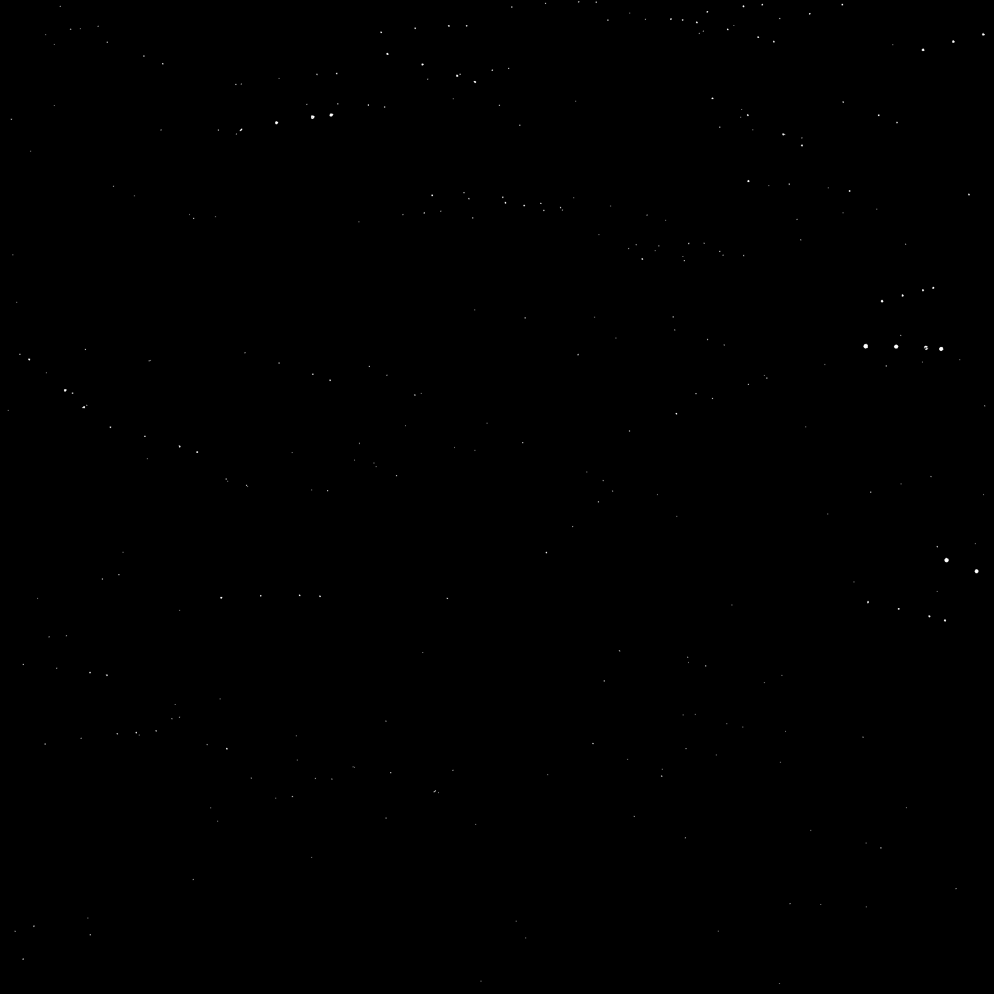
4. This image is the accumulated composite of the difference frames from image set 3. The linear streaks suggest solar system object motion over time. For detail, click and hold the image above to see an exaggerated view. If you can't see all those dots without clicking it'd be really helpful to make your browser wider or find a larger screen to view this analysis on.
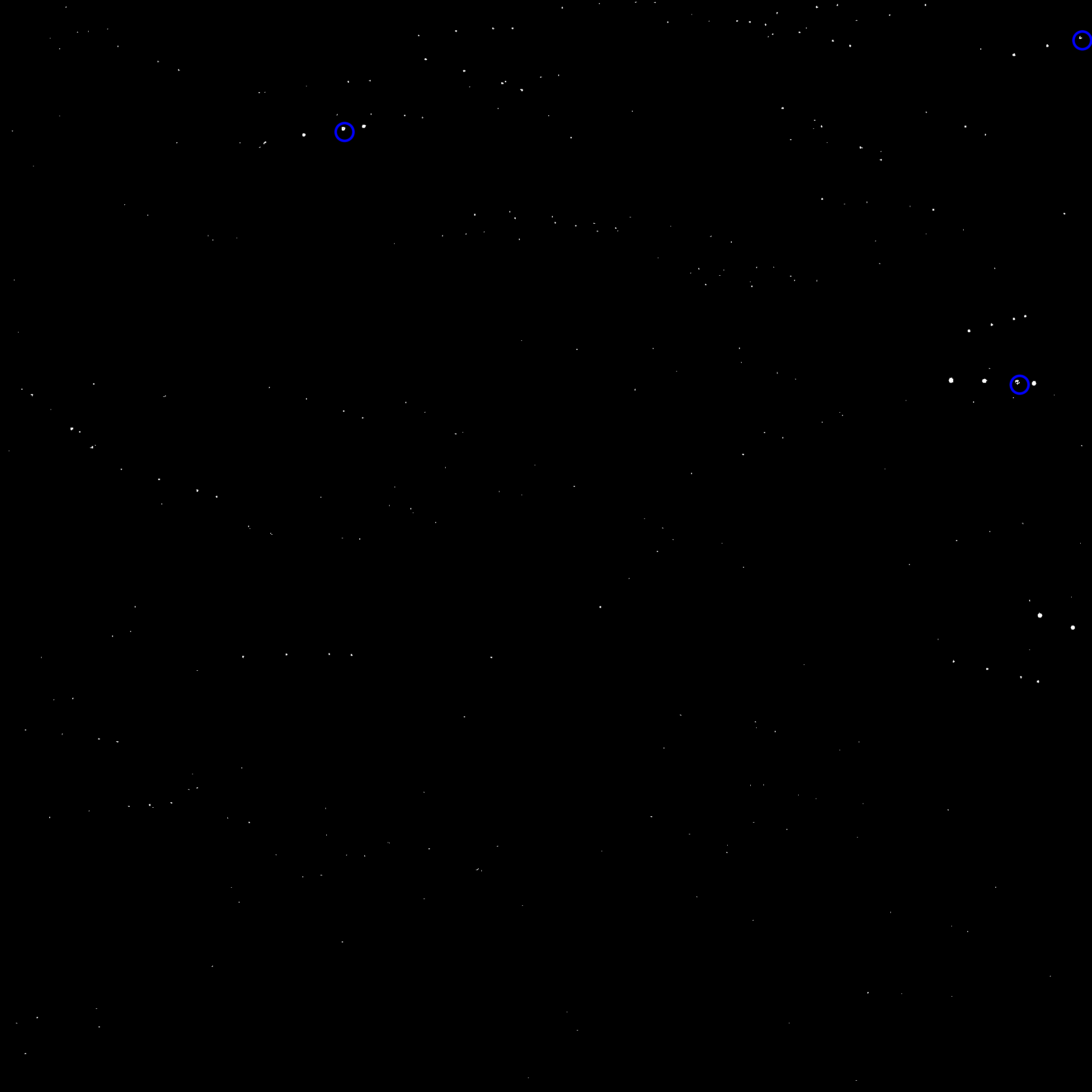
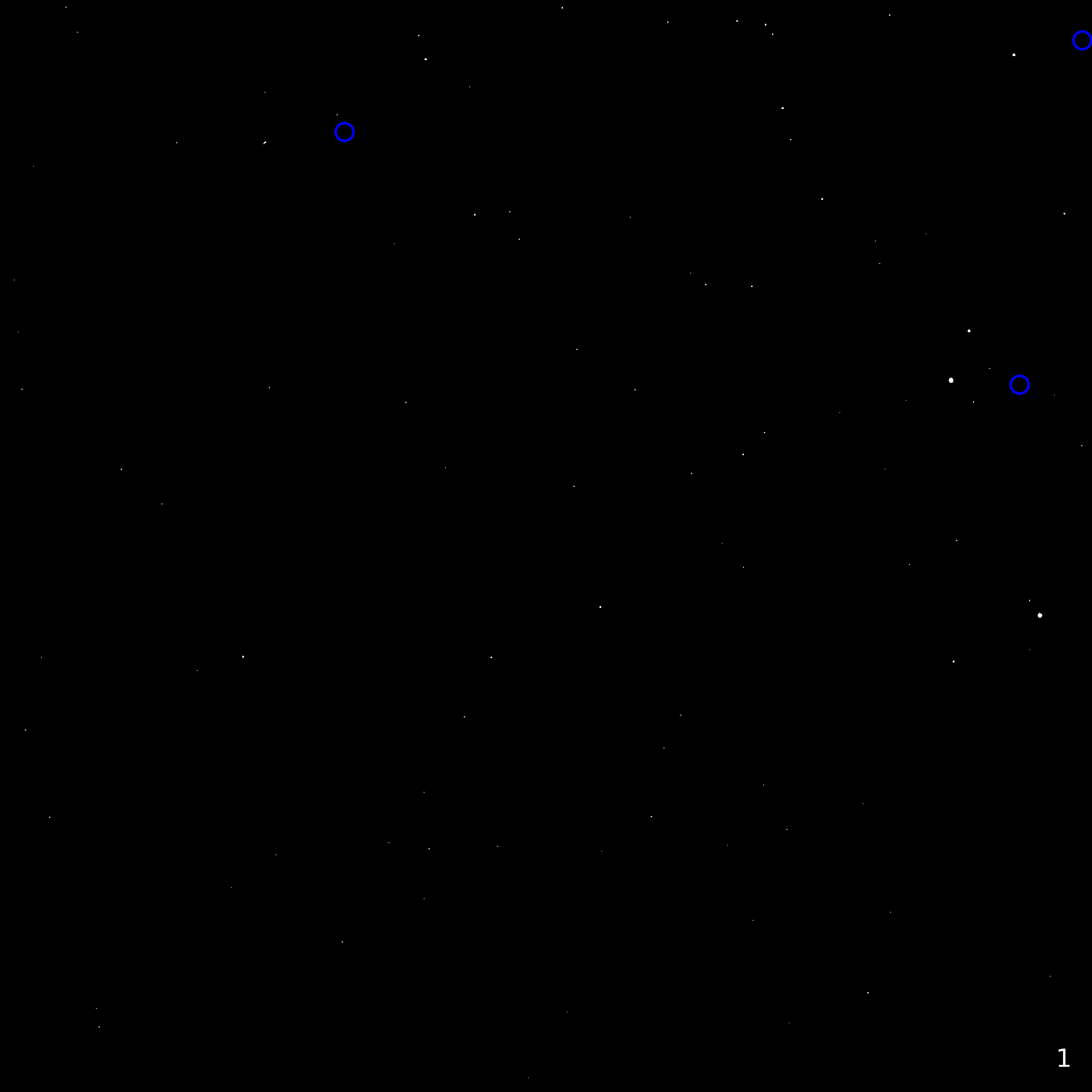


5. These frames are the same as image set 3 except I've plotted blue circles for JPL small body identified objects on the date of frame 3. I selected objects with magnitude < 14 from JPL and only plotted circles where the JPL position was within 6 pixels of one of my detections. Given the 4 asteroids JPL tells me are within this frame at or below magnitude 14, 3 are within this 6px position error tolerance. You can see them pass through the blue circles in frame 3. The circled matches also happen to be the largest blobs and correspond to visible movement in image set 1 which is what one would expect of the brightest objects. Click and hold the image for the streaks view. More in the technical notes below.
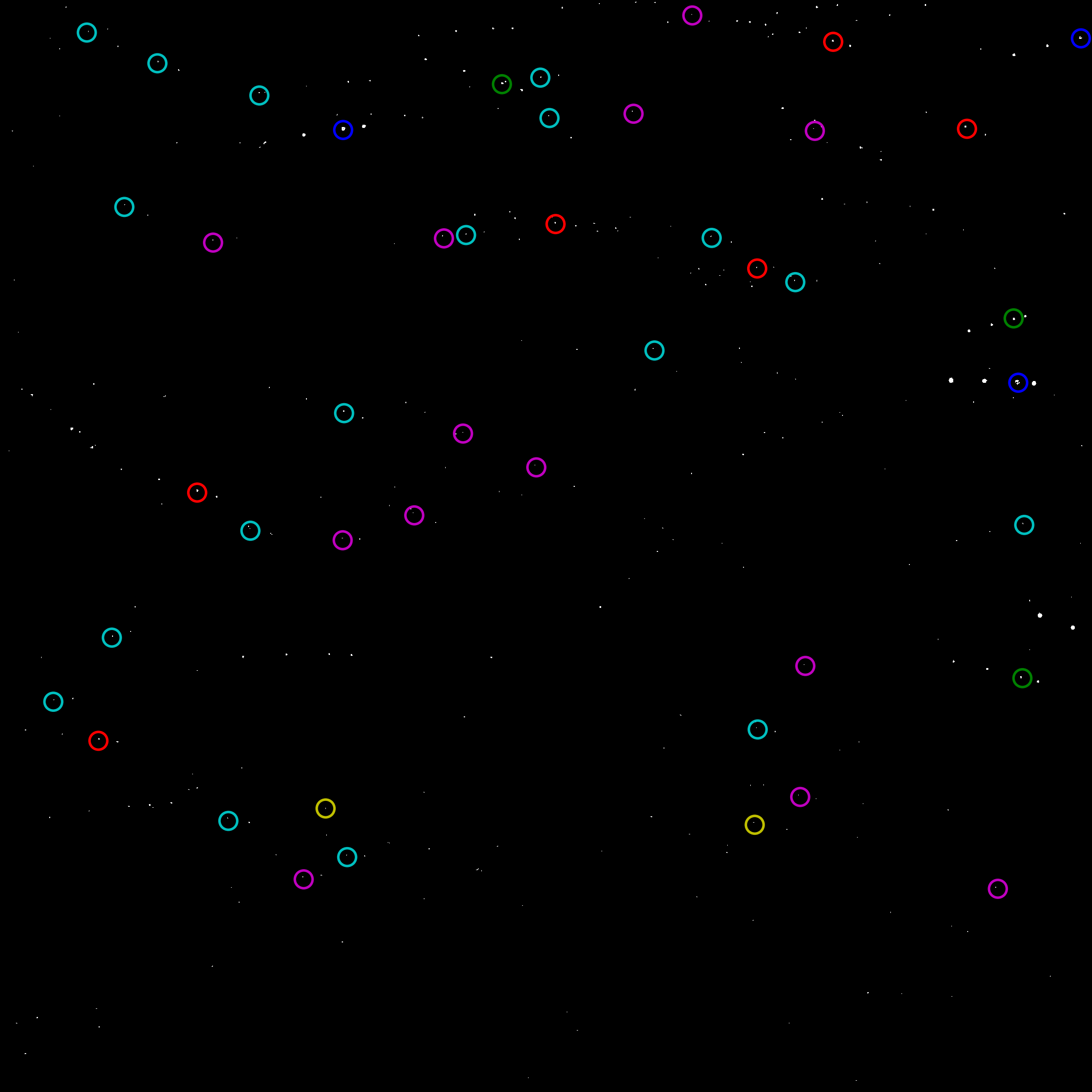

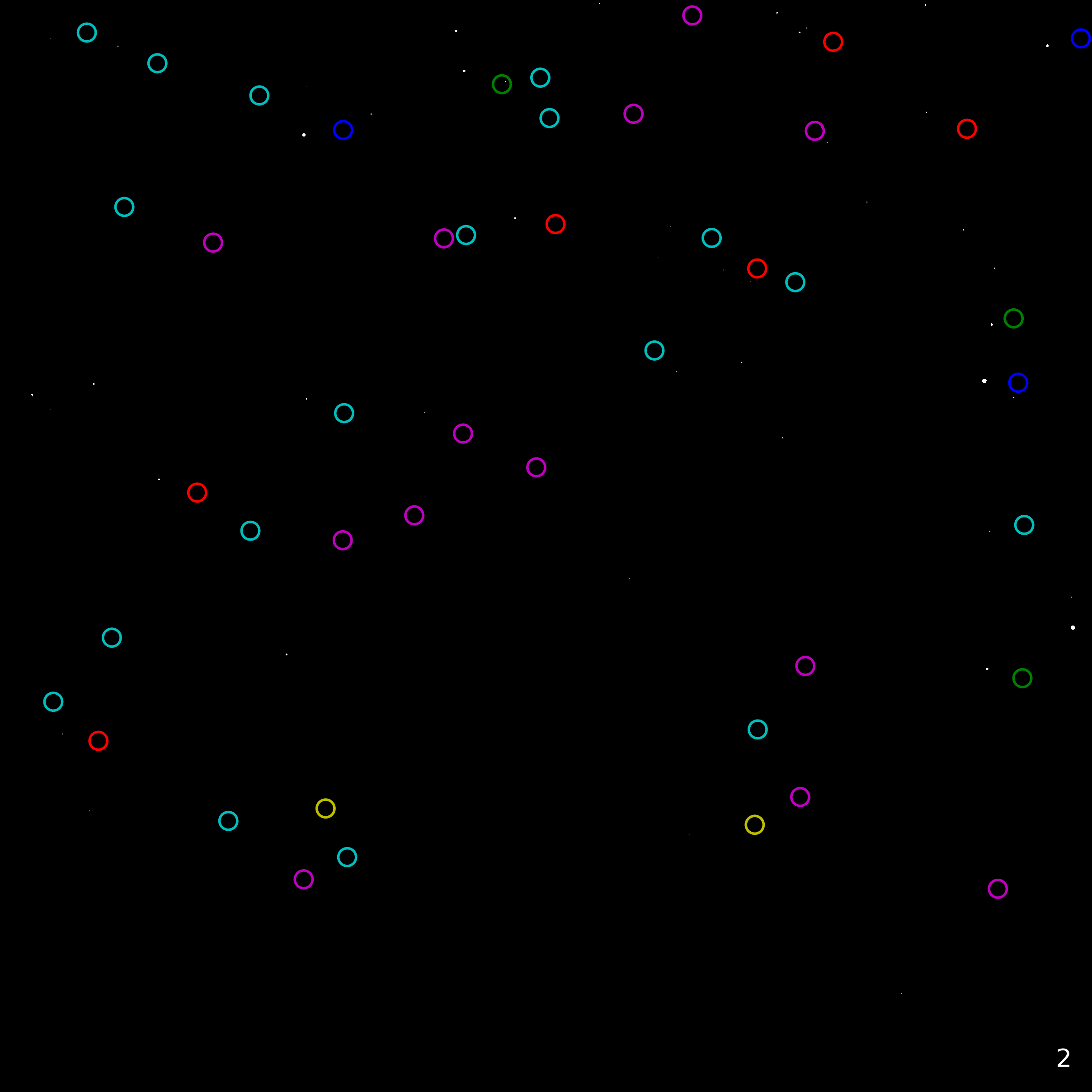

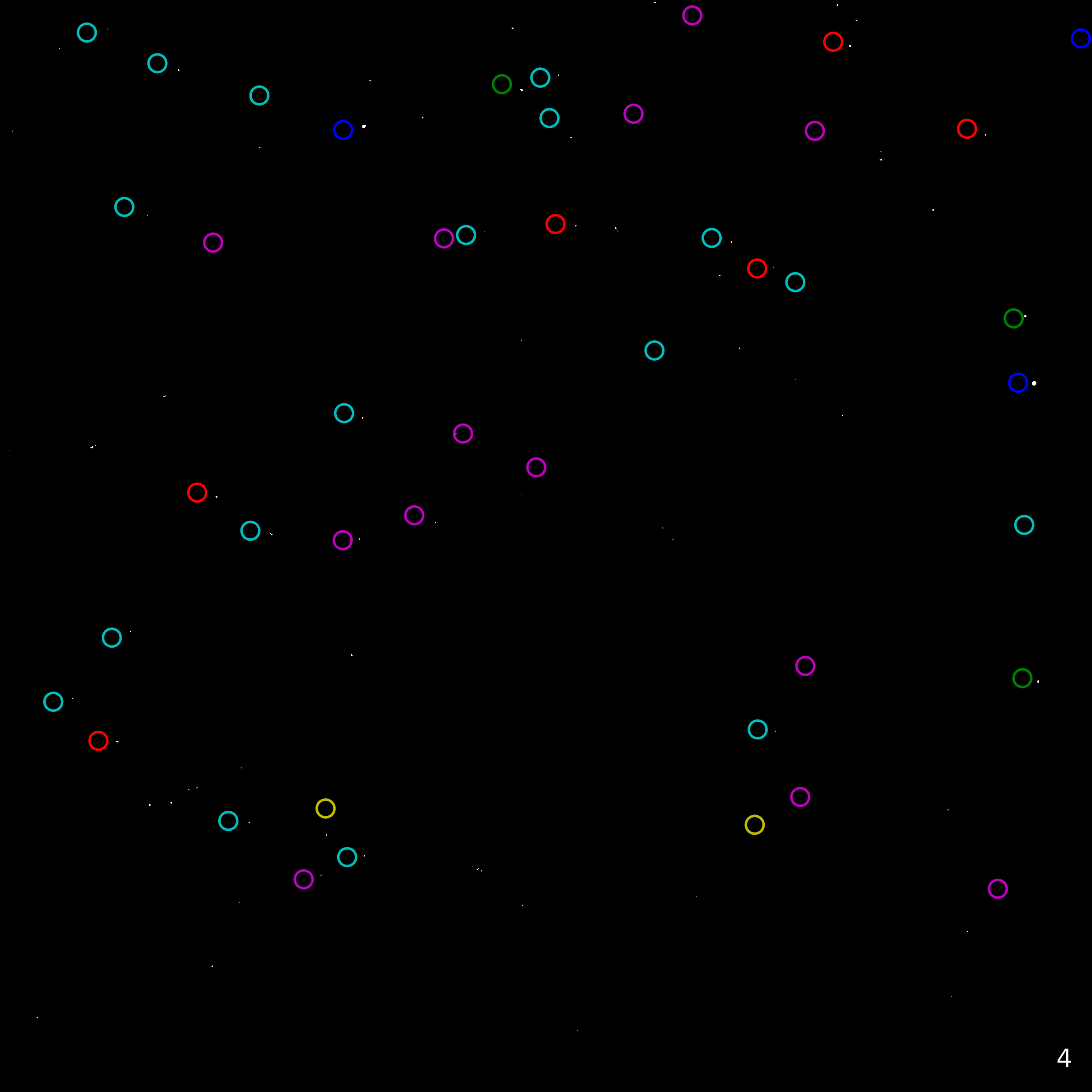
6. Here I've used the 3 objects identified in image set 5 to calibrate the position error of the JPL solution (the error is not JPL's of course, it's most likely the observer location and/or time being incorrectly specified by me by a small amount). The circles are once again expected positions of known objects for frame 3 that correspond to a detection. Note the 3 objects in the blue circles are now close to dead center - that's the calibration adjustment. With this calibration and the same 6px error tolerance I can now match the 45 circled objects with the JPL magnitude limit request raised from 14 to 19. The different colors correspond to the visual magnitude of the objects and are as follows: 13, 14, 15, 16, 17, 18. Higher values are dimmer objects. Click and hold the image for the streaks view. Here is a link to frame 3 if you want to see the full size image. Again, more in the technical note for this image set below.
Image set technical details:
Image set 1: The original images can be obtained via this script. These are somewhat arbitrarily chosen sector 1; camera 1; CCD 3 frames (the closest to the ecliptic). I just looked for frames that were mostly free of artifacts and that had visible object motion to try to detect. You might notice there are 7 frames referenced in that script rather than the 4 I present in image set 1. I'll describe how the 7 frames were reduced to 4 in the notes for image set 3. I took these original 7 images and brightness matched them to a preliminary template calculated as a simple pixel-wise median of the 7 images. Brightness matching minimizes the difference image deltas with respect to a benchmark image (the preliminary template in this case) via a least squares fit. I didn't show the unmodified original frames because to the eye they look imperceptibly different than the brightness matched images. Showing both felt redundant.
Image 2: This is the static sky template that will be used for image differencing. It is calculated as a trimmed max of the stack of the 7 brightness matched original frames. Trimming removes the highest pixel value from the stack of images (again on a pixel by pixel basis) and I then I keep the maximum of the values remaining for each pixel. Next I threshold this template at 3σ to generate a thresholded template. Finally I take the pixel-wise max of the initial template and the thresholded template as the final template. This last step ensures the brightest stationary sources are fully masked while still preserving intermediate values elsewhere.
Image set 3: The difference images in image set 3 are calculated by subtracting the image 2 template from the image set 1 frames and then thresholding. Here's where the frames are reduced from 7 to 4. This is essentially a noise reduction feature. I count the detected sources in each difference frame and then discard frames with significantly larger source counts. This leaves me with the 4 frames I'm showing. When you're working with a dataset like TESS with many repeat observations, discarding data is a viable option. I'll also mention that I tried this process without brightness matching and there was a big difference in the source counts I got from the difference frames. Brightness matching reveals far more sources in the difference images than non brightness matched difference images. It also allows you to reduce the thresholding parameters and reject less signal. These difference frames are thresholded at 1.5σ. It may be useful to go lower even in future studies.
Image 4: This streaks image is just a useful way to visualize the detection trajectories over time. As mentioned above, this image is the accumulated detections from image set 3 rendered as a single composite image. Seeing all the detections laid down in one image reveals linear features that likely correspond to solar system object motion in time.
Image set 5: The motivation for this image set is to identify the brightest objects in the difference frames without throwing hundreds or thousands of known objects up against the 96 detected sources in my difference frame and then say: hey, some of these dots are in the same place! Instead I wanted to confirm the intuition that the brightest (and visually largest) sources in my difference images corresponded to the brightest objects according to JPL. This image set certainly seems to validate that. Using a relatively tight position error tolerance of 6px I can match 3 out of the 4 JPL specified bright objects to sources in my difference image for frame 3. If I loosen up the tolerance I can also match the fourth, but I didn't want to make the position error tolerance too high as I will be using these more precise matches to calibrate matches I will make in the next image set.
Image set 6: For these frames I've used the matches from image set 5 for calibration. That is, I've taken the average x and y pixel offsets of my matched detections from the JPL calculated pixel locations and used this average difference as error correction. The calibration is applied by removing this average detection pixel difference from the calculated JPL pixel position. Specifically, the offset is [-3.75195921, -2.69654259] pixels. With this calibration applied you can see that the blue circled detections are now centered within their circles. From here I open up the matching to all 597 objects returned from JPL with a magnitude of less than 19 within this frame. I keep the position error tolerance at 6px and can now match 45 out of my 96 potential detections in frame 3. The dimmest object I was able to match with these constraints was 18.8. To further validate this technique I tried matching the JPL objects for frame 3 to both frame 2 and frame 4. There were no matches, as one would expect.
Matched detections:
For this analysis I'm only going to claim confirmed observation of the 3 objects I highlighted in image set 5. I'm confident that most if not all of the matches in image set 6 are valid and that there are even more beyond the 45 matches that I didn't identify. For instance, if I loosen up the error tolerance a bit I can get 87 matches out of my 96 potential detections for frame 3. But this is a somewhat sloppy way to identify solar system objects and I want to improve the process before I start making claims about that many objects at once. With that, here are the blue circled frame 3 objects as shown in image set 5 from left to right.
| Object ID | Name | Visual Magnitude |
|---|---|---|
| 81 | Terpsichore | 12.1 |
| 196 | Philomela | 11.0 |
| 844 | Leontina | 13.9 |
Other process notes:
- I didn't apply a PSF deconvolution to these images. I tried some simple parametric PSFs, but all of the images looked visibly worse and I could tell that I was going to be able to detect at least some objects with the unmodified images anyway. I wonder if there are PSF models out there generated specifically for TESS. Or maybe the deconvolution has already been performed on the full frame images and I just haven't been able to find anything about it yet in the documentation.
- I didn't need to use an expansion mask in the template image for this solution (unused example here with exaggerated contrast for visibility). I think having more frames to build the template from reduces the necessity of this. With only 2 frames in some Allsky detections I sometimes needed to grow the edge of the star mask (i.e. the template image) to fully remove stars in each difference image.
- I didn't use the remove_small_objects() function. It might be useful in the future if I lower the difference frame threshold level, but it doesn't seem necessary here yet.
Ideas & Todos:
- I need to improve my object identification process obviously. I think what I've done here is confirm that I'm not just looking at improbably arranged noise, but I need to get way more precise with my matching and figure out why I'm missing what seem like obvious detections. I think the JPL small body identification tool can work if I can either get it to accept a TESS TLE or somehow represent a applicable topocentric origin for a non-topocentric observer like TESS.
- Investigate PSFs for TESS further (see PRF mention here).
- Totally speculative thought here, but I wonder if slower, dimmer, more distant objects might be resolved by stacking observations closely spaced in time. I am unsure what the relationship between limiting magnitude and image processing is; that is, how much can image processing extend limiting magnitude. Coincidentally, this paper on detecting TNOs with TESS was published after I wrote this note to myself but before I published this analysis. I think I know what my next project is going to be.
- Object linking: I did not attempt it. It's going to have to be more sophisticated that the naive sequential, spatially constrained linker I was using if there are going to be so many detections to link. If I get JPL object matching working better and remove known objects from difference frames I might be able to get away with simple linking though. But then again it doesn't seem very likely that there will be as yet unidentified objects in my analysis.
Discussion:
I'm encouraged by how much of the work that I've done with Allsky cameras has translated directly to TESS full frame images. The Allsky process required image alignment which meant you to had to pay close attention that linear features like those in streaks images above weren't actually bad pixels moved along a path by the registration process. TESS images, however, don't need to be registered and the images are already calibrated, so there is far less concern that I'm generating those kinds of features by the process itself.
I'm also encouraged by the preliminary matching process I've begun. It's already way better than the look very closely at Stellarium technique I used for the Allsky objects like Ceres because I now have WCS data for the field. Nevertheless, I'm considering all matches beyond the first 3 in image set 5 to be likely, but tentative. I don't want there to be any question about the objects I'm identifying.
Even if I was able to match all 96 of my detections there would still be 501 undetected objects below 19th magnitude somewhere in frame 3, so there is plenty of work left to do to improve recall. Granted, if I'm matching even some objects down to almost 19th magnitude with this preliminary wide-field study I'm pretty happy. There are still obvious non-dim objects that I haven't matched too, so first things first. For instance, right above the left-most yellow circled match there's an obvious object moving from left to right in the animated frames. Why haven't I matched that one? Or the many others that I can see that are unmatched with linear trajectories?
I'm tempted to focus on the detection of more objects in these frames and just interate on that component until I can't bring the position error down any further and have identified all or most of my detections. But I think I'm more tempted to look for dim outer solar system objects first - maybe some TNOs. I definitely don't think I can duplicate the TNO detections in the paper I mentioned above, but there are slightly brighter TNOs out there too that may be observable if they've fallen within TESS' observation field yet (they will eventually). Even trying and failing to observe them would be interesting, so that's probably what I'm going to work on next. I expect it will yield improvements that can be applied to this study as well.
Published: 11/13/2019