
HelioLinC-ing a CSS Superfield
In previous work I've investigated Catalina Sky Survey data for individual observation fields. A field is a specified location on the sky that CSS revisits 4 times in one night to gather data in order to identify moving objects within that field. For this study I've built a "superfield" that is a combination of 8 adjacent fields observed on 3 separate nights (4 times per night) over a span of 10 days. The motivation for creating a superfield is that it might allow you to do 'blind' object validation with orbit determination. One night of observational data is not enough to confirm an orbit but (perhaps) 3 nights of data over a 10 day interval might be. This study will investigate that hypothesis.
Building the Superfield
Step one in building a superfield is to define the thing: it's simply what I'm calling a set of observational data that spans multiple fields and nights. For this study I searched CSS fields for the Mt. Lemmon telescope (G96) within 7 days of the January 31st 2022 new moon that were observed on 3 separate nights. There's no database that I know of that contains this information, so I wrote some code that checks the nightly field files CSS publishes to PDS to count how many times a field appeared in this two week interval. At first I thought this might yield individual fields separated randomly on the sky, but instead I found fields that have 3 nights of observations in that time window are adjacent to one another. I probably should not have been surprised by this; CSS' survey strategy is not random after all. When the telescope revisits one patch of sky it also revisits those patches around it too for efficiency sake. In the end, 8 CSS fields for G96 met the 3 separate night observation requirement I specified.
Once you know what fields to investigate, the next step is to generate the sources from the observation data. The process I used is not too different than the one I outlined in a previous study. I considered each field+night combination independently and removed Source Extractor sources within 1" of one another that occurred more than once in that field+night combination as duplicate sources in the same location indicate a likely stationary source. I did not use difference image sources. The result was 1,432,788 sources across 96 observation times (3x4x8). SBIdent revealed that 24,678 of these sources were associated with known objects matched to 1" or less with a collective RMS error of 0.35".
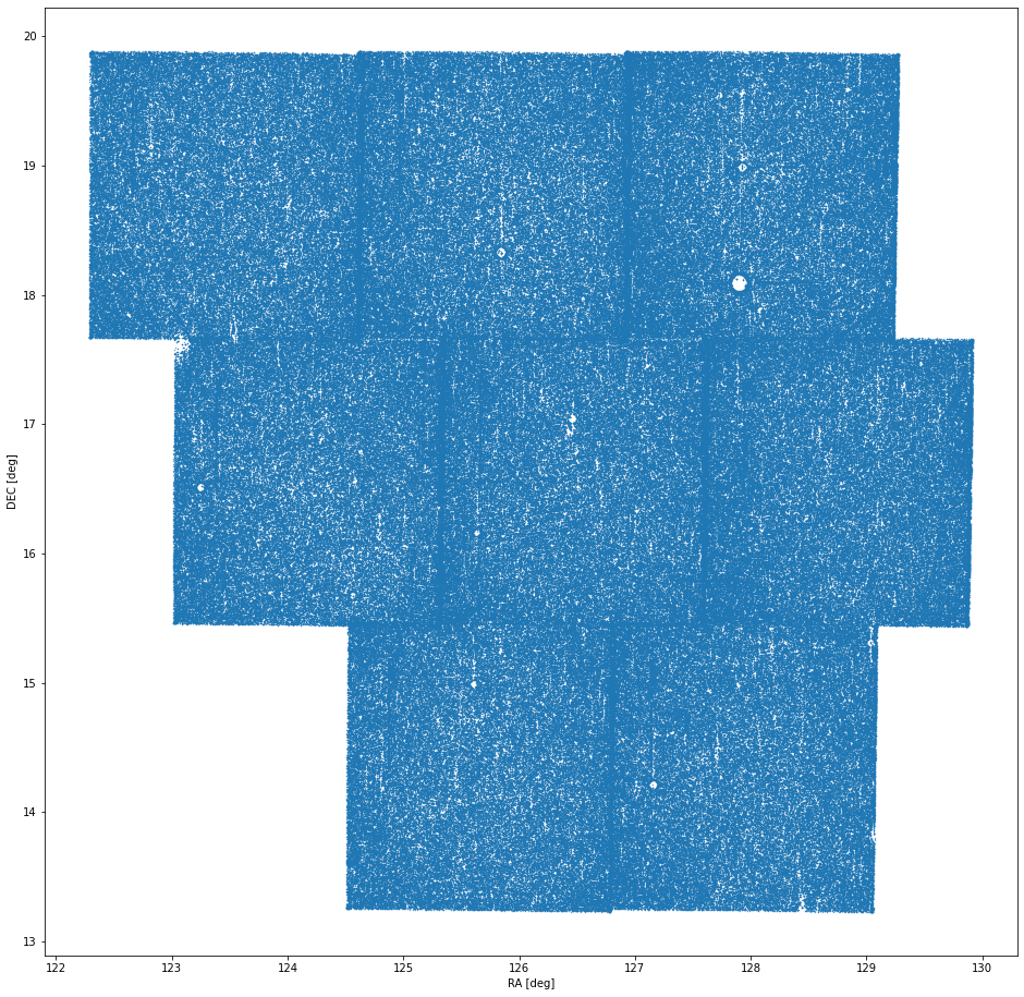
Image 1. 1,432,788 sources extracted from 3 repeat observations of 8 fields over the course of 10 days around January 31st 2022 centered on N16056.
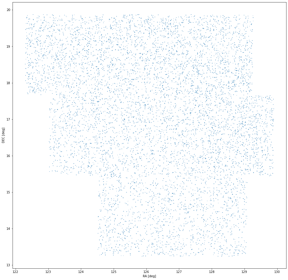
Image 2. The 24,678 sources that match known objects in image 1.
Linking with HelioLinC
Conceptually, HelioLinC is a fairly simple thing. You take pairs of RA/DEC sources that are close to one another in the observational data (tracklets), assert a set of physical parameters for those pairs (e.g. range, range-rate, range-rate-rate), and then propagate the orbit that those physical parameters specify to a common epoch. Propagated pairs that are in close proximity to one another in position and velocity at the epoch yield candidate links that may (with further validation) represent real solar system objects.
For this study I focussed on maximizing recovery of the known objects within the superfield. Being able to find the known objects in a set of observational data is an obvious prerequisite to being able to find new, unknown objects in the data. As such, I've limited HelioLinC's search space to the parameters specified by the known objects in the superfield. Specifically, I created tracklets on sources with implied on-sky angular velocity of up to 0.5°/day and then searched between 1.5 - 3.5 AU using asserted range-rates between -1e-2 AU/d and 1e-2 AU/d. The charts below summarize the recovery results for known objects with this search.
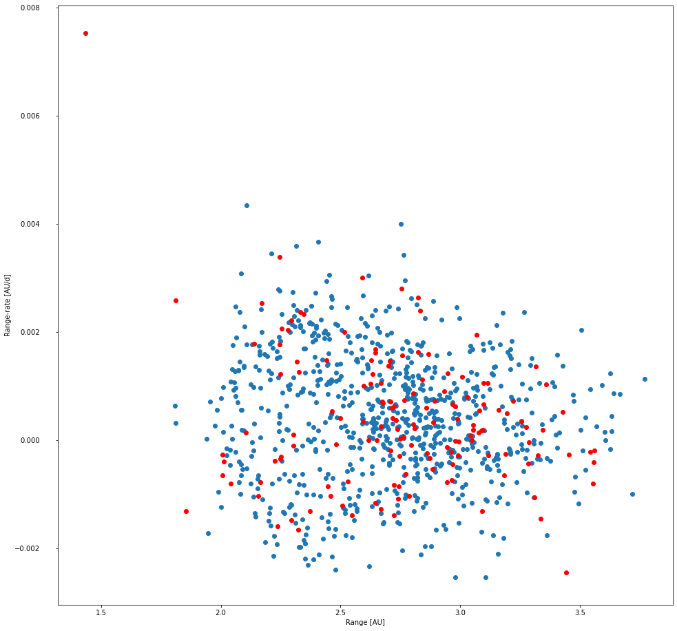
Image 3. Recovered/Unrecovered range vs. range-rate of the known objects in the superfield.
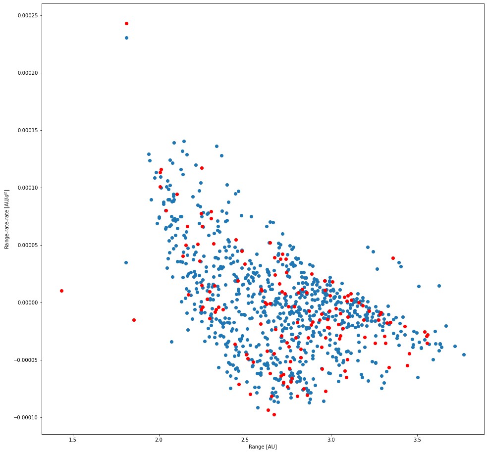
Image 4. Recovered/Unrecovered range vs. range-rate-rate of the known objects in the superfield.
In the two images above, each dot represents one known object that was potentially recoverable from the data. I define a potentially recoverable object to be an object with at least 2 detections per night over 3 nights. There are 930 known objects that meet that potential recovery definition. Blue dots are a recovery and red dots are a failed recovery, meaning HelioLinC was not able to find them.
You'll notice that while HelioLinC is able to recover most objects (84.52% specifically), it by no means finds all of them. I tried many combinations of search parameters to increase the recovery rate and found only marginal improvement. There's a good reason for this which the next set of images will reveal.
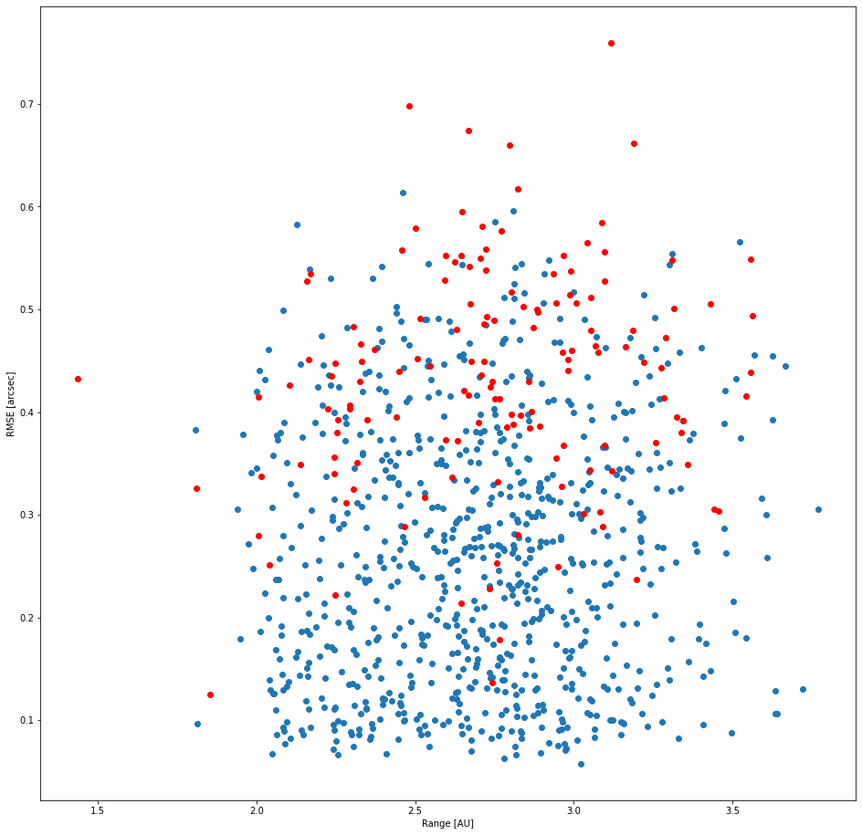
Image 5. Recovered/Unrecovered range vs. RMS error of known object detections in the superfield.
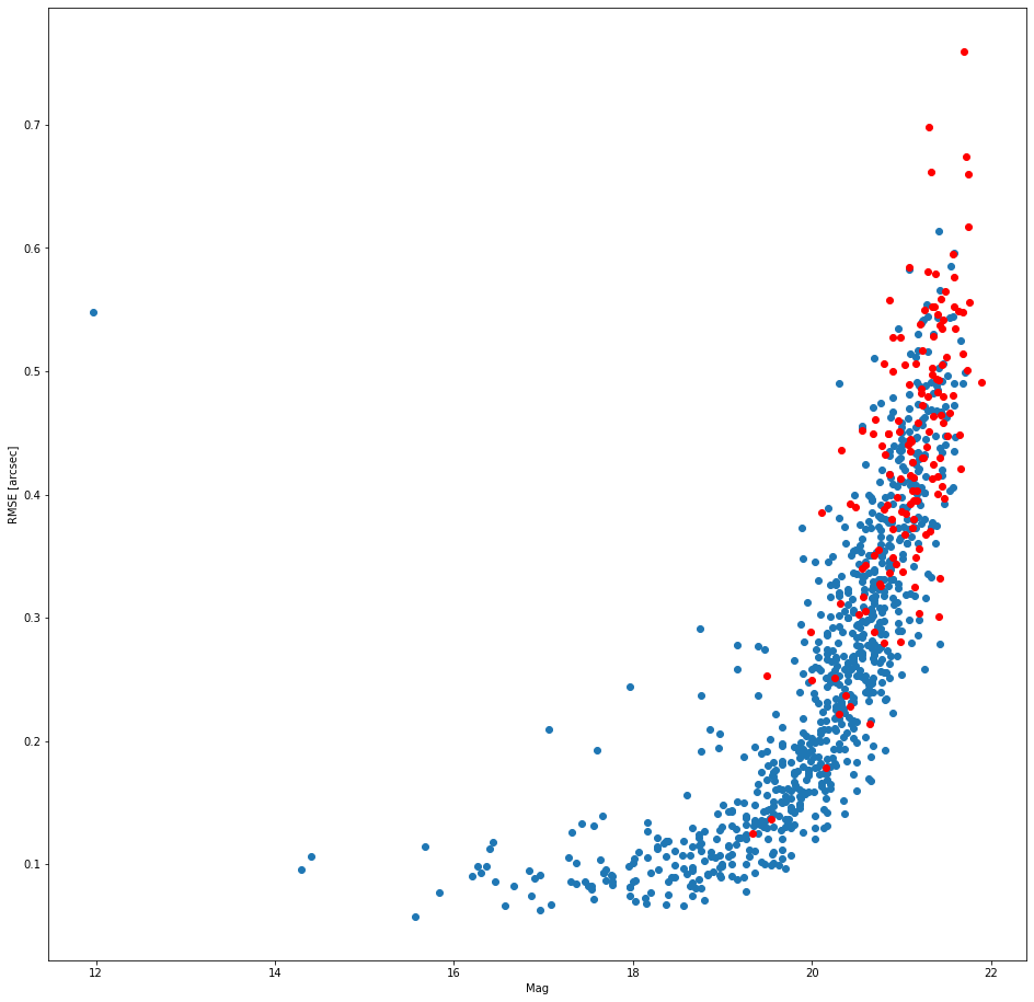
Image 6. Recovered/Unrecovered visual magnitude vs. RMS error of the known objects in the superfield.
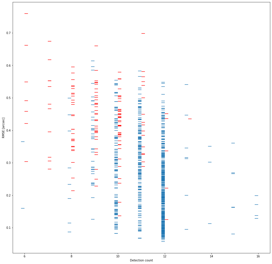
Image 7. Recovered/Unrecovered count of detections in a known object link vs. RMS error.
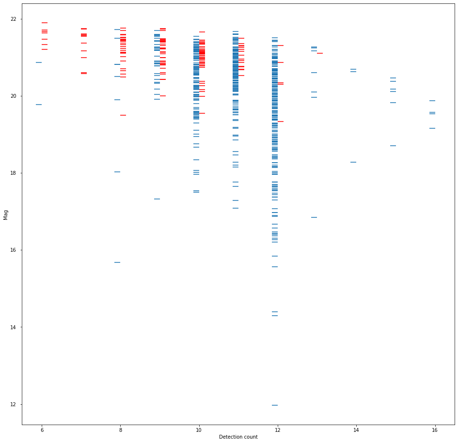
Image 8. Recovered/Unrecovered count of detections in a known object link vs. visual magnitude.
The bulk of the known objects that HelioLinC was unable to find were 1) objects with relatively poorer astrometric accuracy (higher RMS error) [image 5], 2) dimmer objects (which also necessarily have poorer astrometric accuracy) [image 6], and 3) objects that had fewer detections in the observations thus fewer potential combinatorial opportunities to cluster in quantity [images 7 and 8].
The takeaway here is that HelioLinC has more difficulty with high astrometric error and low detection counts. I think there's a bright side to this story, however. Look at the count=12 column in image 7 and then scan up to the highest blue horizontal line (the worst RMS recovery that HelioLinC found for that count). Now look left to the lower count data. You can see that with more detections HelioLinC is able to recover more objects with higher astrometric error. Image 8 shows the same basic thing. If you get more detections you can link dimmer objects with poorer astrometry. This tells me I should probably look across more time (beyond 3 nights) in future work.
The table below summarizes the overall recovery results. Note that 12 detections (4 on each of the 3 nights) has an almost 99% recovery rate.
Table 1. A summary of known objects recovered by HelioLinC
| Detections | Recovered | Recoverable | Percent |
|---|---|---|---|
| 6 | 2 | 9 | 22.22% |
| 7 | 0 | 11 | 0.00% |
| 8 | 8 | 35 | 22.86% |
| 9 | 35 | 70 | 50.00% |
| 10 | 122 | 164 | 74.39% |
| 11 | 179 | 195 | 91.79% |
| 12 | 420 | 425 | 98.82% |
| 13 | 7 | 8 | 87.50% |
| 14 | 3 | 3 | 100.00% |
| 15 | 6 | 6 | 100.00% |
| 16 | 4 | 4 | 100.00% |
| Total | 786 | 930 | 84.52% |
Orbit Determination and Bootstrap Filtering
The confirmation of known objects above were made with ephemeris data from JPL (via SBIdent). Ideally we'd also be able to confirm objects (both known and newly discovered unknown objects) by orbit determination as well. Things are not quite that simple, but for the case of unknown objects we obviously can't rely on the known catalog to validate them. And unfortunately, not all candidate links that HelioLinC (or any other linker) produces and that OD solve will be real physical objects. There are simply too many ways to construct a valid and well fitting orbit from the reasonably short arcs you are working with for the linking problem.
Image 9 below illustrates the challenge. First some definitions. All of the small horizontal ticks represent an OD solve for a HelioLinC generated link at the RMS indicated on the y-axis. All of these solves are less than 1", which is generally quite good. The x-axis groups these solves by the number of detections. Green ticks are solves for known objects with no confusions (they contain no erroneous detections nor are they crossed with other known objects). Blue ticks are unknown solves — there are no known object detections within these links. Red and orange ticks are variations of impure solves. Red ticks are 2 or more known objects that are crossed (e.g. think of a link with Ceres and Vesta detections in it). Orange ticks are solves with unknown detections but also at least 1 known object in the link.
Ideally, these red and orange ticks would not solve with OD because they are "wrong" in some sense. The good news is that we know they are all wrong, so we don't have to accept their OD solutions as validation. Additionally, I propose we can use their wrongness as a way of bootstrapping an OD filter that is more effective than a simple RMS filter alone.

Image 9. All OD solves less than 1".
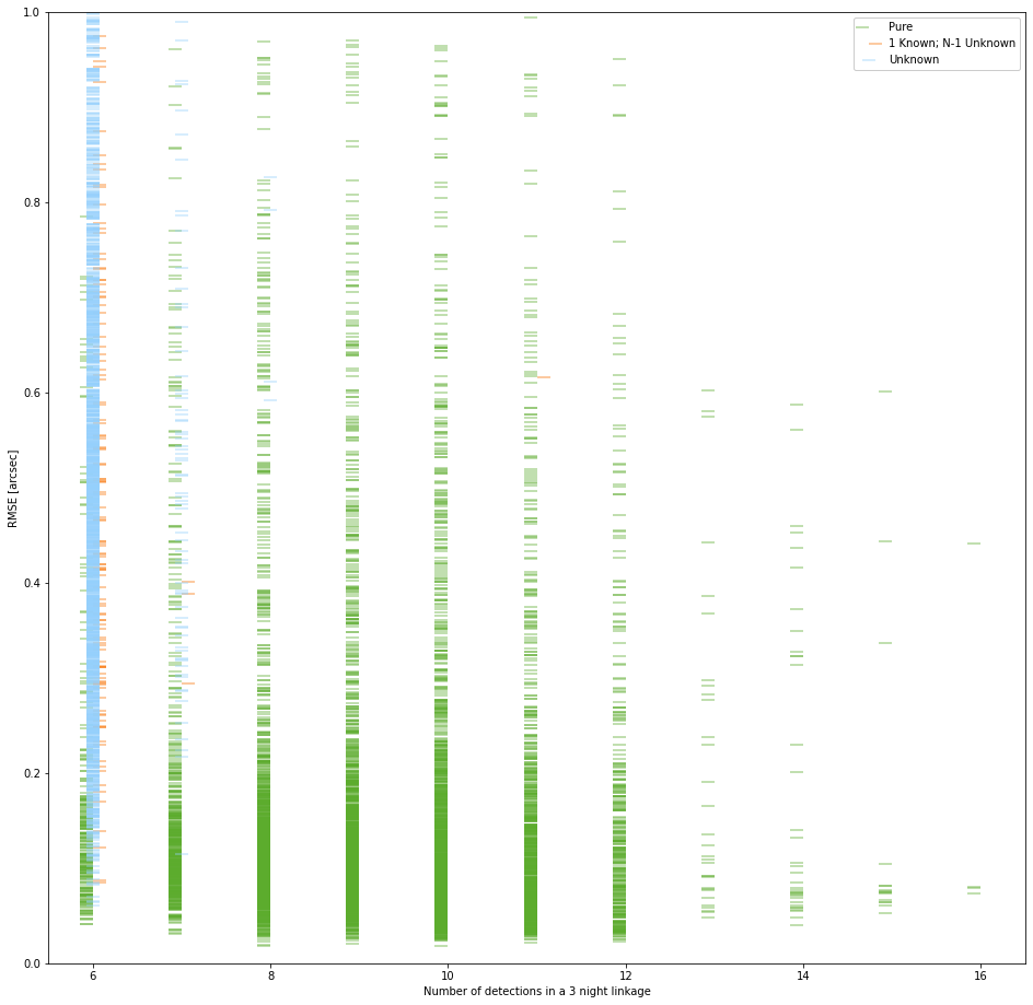
Image 10. OD solves less than 1" with only "1 known; N-1 unknown" type impures shown.
Image 10 above is a subset of the data shown in image 9. The pure (green) and unknown (blue) solves are unchanged. The orange solves are a subset of the unknown impures which contain 1 known object match and all the rest of the link is unknown. There are simply too many blue ticks and they can not all represent new undiscovered objects. I suggest that the "1 known; N-1 unknown" links are the most adjacent thing which we can know is bad to an N unknown sized link that is bad which we can't know is bad. To say this another way, if we had a (say) N=6 link that was all unknown detections, we could not know that it was bad from catalog information. But a 1 known; 5 unknown link we can say is bad from catalog data. Thus, the idea is that we can use RMS solve for "1 known; N-1 unknown" solves to inform our decision about RMS thresholds for filtering unknown links of size N.
Bootstrap filtering, as I'm calling this concept, uses the smallest RMS solve value for a "1 known; N-1 unknown" for a given link size (N) as the threshold for filtering. The table below summarizes three different filtering methods. One is a simple RMS filter of 1" with no known object catalog rejection; one is bootstrap filtering with impure rejection from catalog information, and the last is a tighter RMS filter (0.5") requiring more detections in a link (8) that also uses the known object catalog to reject impure links.
Table 2. Three OD filtering techniques for object validation
| OD Filter | Pure Solves | Impure Solves | Unknown Solves | Known Objects Validated |
|---|---|---|---|---|
| 6 detections; 1" | 6,101 | 2,120 | 2,050 | 780 |
| Catalog rejection + Bootstrap | 5,781 | 0 | 18 | 768 |
| Catalog rejection; 8 detections; 0.5" | 4,882 | 0 | 0 | 727 |
To be explicit, we want to use OD to do two things: 1) validate the links associated with real objects; 2) reject candidate links that are not associated with real objects. The table summarizes how three different techniques perform in this task. The first, 6 detections; 1", shows that an RMS filter by itself for the 6 detection minimum case validates the most known objects (780 out of the 786 HelioLinC recovered). However, you can see that it fails to filter thousands of impure links (which are bad) and also allows thousands of unknown links (which are simply too numerous to be believed). At the expense of 12 lost known object validations, catalog + bootstrap filtering rejects all impures (by definition really) and allows 18 unknown solves — a more approachable and believable amount of potentially new objects to consider. The third filter, catalog rejection for 8 detections or more with an 0.5" RMS filter, validates 727 known objects but leaves no solved unknown links to investigate.
Bootstrap filtering seems to strike a balance between filtering too much and filtering too little. It validates almost as many objects as the simple 1" RMS filter and allows a plausible amount of unknown links with very tight orbit fits for further consideration. I'll show some of them in the next section.
Visual Validation
Before I explore individual objects, I want to show what the on-sky tracks for the known objects look like compared to the tracks for the bootstrap filtered links. The children's drawing in image 11 shows all of the known object OD solves. Image 12 shows the bootstrap solves. The numbers next to the bootstrap solves are the internal IDs I use to reference them. What's interesting to notice here is how linear all of the known object tracks are while many of the bootstrap tracks are not. In principle there is nothing wrong with this. One of the strengths of the HelioLinC approach is that it can find objects that have non-linear motion on-sky, but I am unsure if this quantity of non-linear tracks should be expected. This is something I'll be paying attention to in future work.
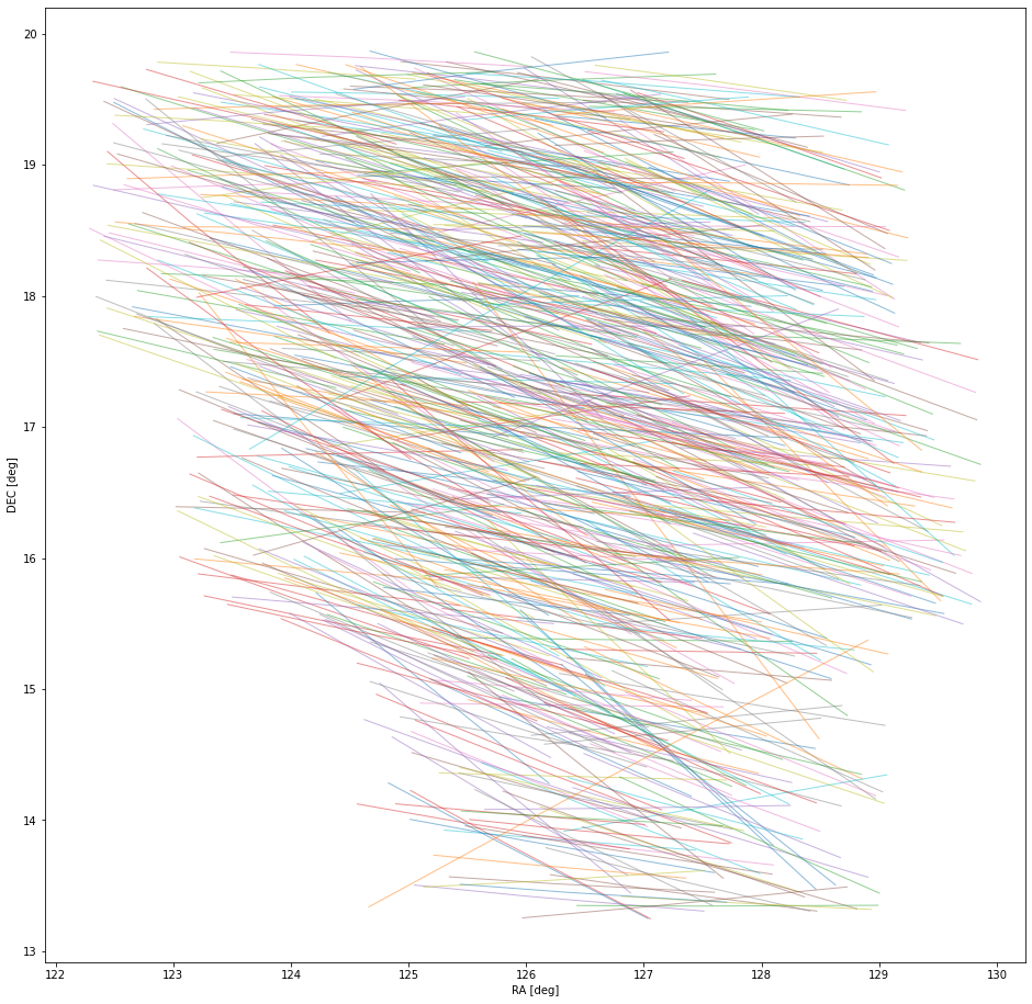
Image 11. All of the known object OD solves in RA/DEC space.
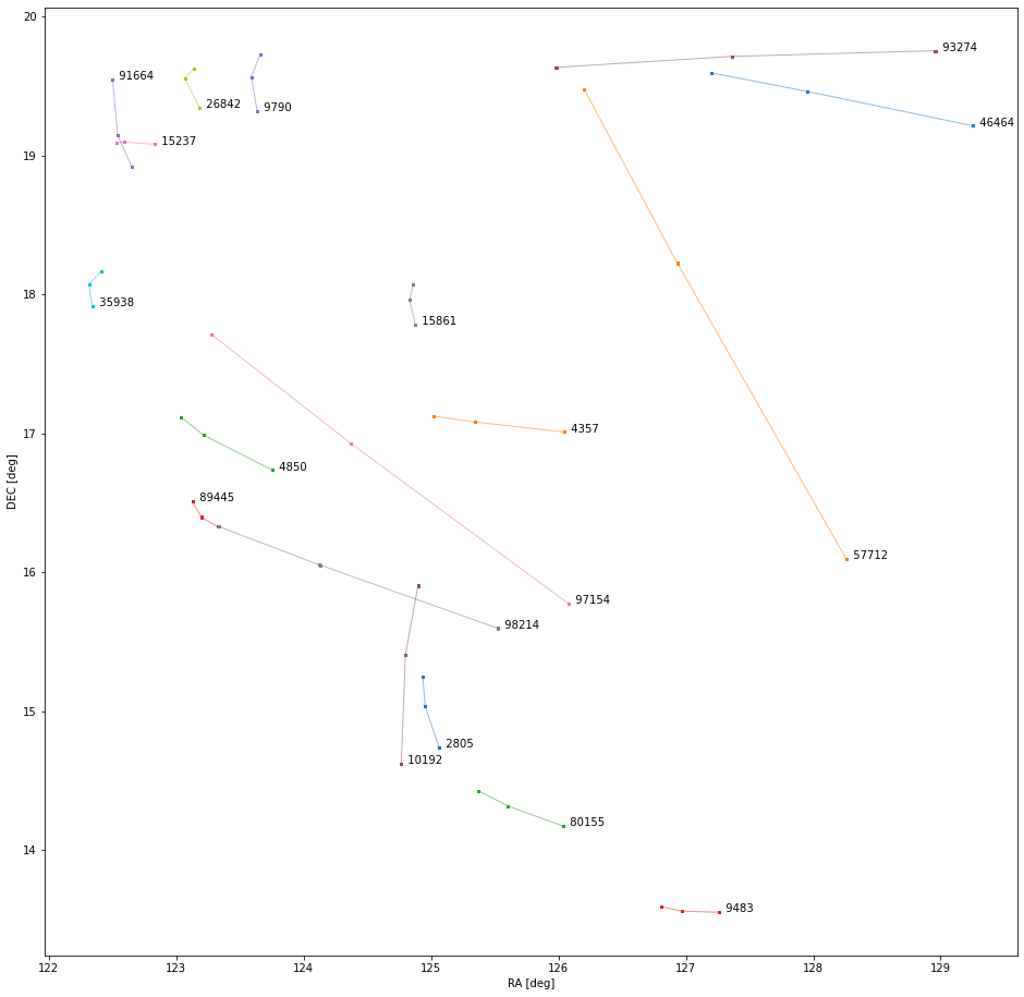
Image 12. The bootstrap filtered unknown OD solves in RA/DEC space.
Next let's look at a couple of images of known object detections from the superfield before we start looking at unknown objects in order to get familiar with the visualization technique I'm using for moving object detection. This technique was suggested to me by Eric Christensen at CSS as an alternative to the more naive visualization I was using in my last NEO study. In that previous work I was just showing the location of the detection in each of the frames where a detection occurred. These images (below) show the location of the detection at the time of detection on the diagonal. Each column of the off-diagonals are the detection location for times other than the detection time in the candidate link. You want to see a detection (black) on the diagonals and non-detection (white or noise) in the rest of the column. To make it more straightforward, I've added a green square to the cells that you want to see a center detection and a red square to the cells that you do not want to see one. There are no observations for the field+time combination in the empty squares.
Image 13 shows 2008 KA39 (mag: 20.5), an average known object detection for CSS. It's quite apparent that there is something present along the diagonal that is not present in the off-diagonals. This presence along the diagonal and non-presence in the off-diagonals is the visual validation of a moving object because it shows that something is present in a location at one time and not present at the same location at other times, thus moving.
Image 14 shows 2022 AF42 (mag: 21.7), the dimmest known object found in this superfield. The diagonal/off-diagonal relationship is still there, but it's more difficult to see. Incidentally, 2022 AF42 was discovered by CSS on a prior night, but it is perhaps microscopically noteworthy that the two bottom-right detections on 2022-02-05 were not part of CSS' MPC submission because they were the only two detections on that night and CSS requires 3 detections minimum to form a link. HelioLinC was able to link across multiple nights of the superfield and could thus tack on the two additional detections.
-11.png)
Image 13. Know object 2008 KA39 (V: 20.5).
.png)
Image 14. Known object 2022 AF42 (V: 21.7).
Finally, let's look at some of the bootstrap filtered unknown candidate links HelioLinC found. There are a handful that look promising to me, but I'm just going to highlight two that are near the top of that list for three reasons. 1) they are relatively longer at 8 detections each, 2) they have linear tracks [see image 12], and 3) they both have a 100% p_NEO score in their find_orb OD solutions [CSS' mission is NEO discovery]. I haven't studied the accuracy of p_NEO scores for short arc OD solutions extensively though, so I don't put too much stock in that categorization. Both candidates are hanging out at or near the limiting magnitude of the telescope and thus should resemble the faint detections of image 14. I think at least a subset of the detections in both image 15 and 16 look valid, but I'm definitely going to need a second opinion on that from the experts at CSS.
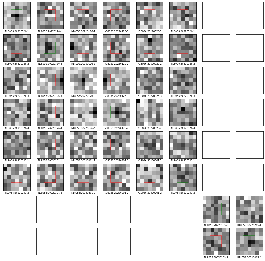
Image 15. Unknown candidate 93274 - RMS: 0.59”; V: 21.6; V𝜎: 0.5.
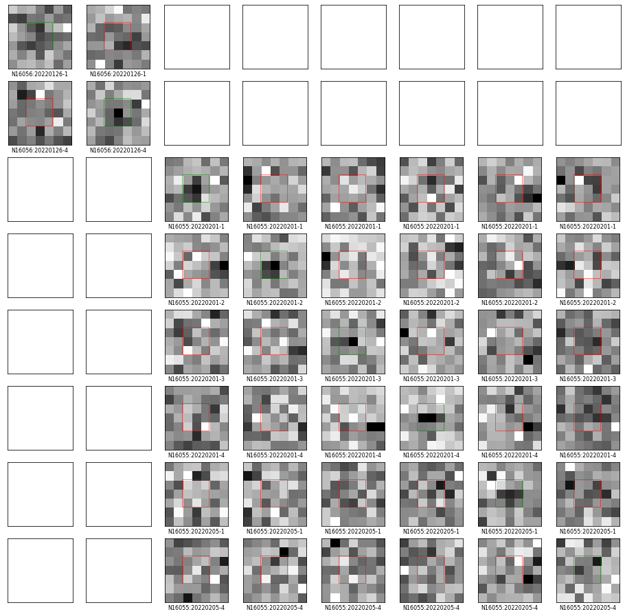
Image 16. Unknown candidate 98214 - RMS: 0.83”; V: 21.6; V𝜎: 0.48.
Conclusion
At the beginning of this study I said that I would be investigating the idea that a superfield with observations on 3 separate nights would allow 'blind' object validation via orbit determination. I think the answer is probably: no, not really — at least not for short links of 6-8 detections. If you get a 12 detection unknown candidate link maybe you could validate that with OD alone, but I saw none of those in this study. The interesting links I found with bootstrap filtering were short enough that they still require visual validation.
Still, I think this superfield direction is the right one for numerous reasons. For one I think it's a complementary approach to what CSS is already doing with single night searches rather than a conceptual duplication of their search technique. While HelioLinC has demonstrated an ability to work well with single night searches, I don't have the capacity as an individual to scale that up to search the hundreds (thousands?) of fields that CSS observes each night and to then visually validate all of the candidate links it produces. It's also quite presumptuous to think that my HelioLinC implementation would perform any better than the techniques CSS has honed over the years as the premier NEO survey for single night searches. But maybe I can search their data in a different way and uncover objects with fewer than 3 detections per night by linking across multiple nights.
For these reasons I think extending the superfield concept to as many nights as I can is the way forward. That way I can rely on orbit determination to reduce the false positive count to something more approachable for shorter links, and more nights of data will eventually yield links that OD alone will validate. The shorter links will always require inspection judging from this work, so visual validation won't be going away either. While I can't visually validate hundreds or thousands of links per night, I think bootstrap filtering (or something like it) can keep the interesting candidate list small enough to work over larger frame+time intervals.
Finally, the superfield approach opens up the potential for discovery of more solar system objects than just NEOs, and I'm quite interested to see what other categories of objects a larger superfield with more nights of data can find. I think I have to try to build a bigger superfield next.
Published: 11/13/2022